General Applications of Neural Networks
Lab 1: Neural Network Linearity

Instructor: Wesley Beckner

Contact: wesleybeckner@gmail.com

---

In this lab we will compare the FFNNs to simple linear models

---

Data and Helper Functions

import plotly.express as px
from sklearn.datasets import make_blobs, make_moons
import pandas as pd
import numpy as np
import matplotlib.pyplot as plt

X, y = make_blobs(random_state=42, centers=2, cluster_std=3)
X, y = make_moons(random_state=42, noise=.05, n_samples=1000)
px.scatter(x=X[:,0],y=X[:,1],color=y.astype(str))

def plot_boundaries(X, clf, ax=False):
  plot_step = 0.02
  x_min, x_max = X[:, 0].min() - 1, X[:, 0].max() + 1
  y_min, y_max = X[:, 1].min() - 1, X[:, 1].max() + 1
  xx, yy = np.meshgrid(np.arange(x_min, x_max, plot_step),
                        np.arange(y_min, y_max, plot_step))

  Z = clf.predict(np.c_[xx.ravel(), yy.ravel()])
  Z = Z.reshape(xx.shape)

  if ax:
    cs = ax.contourf(xx, yy, Z, cmap='viridis', alpha=0.2)
    ax.scatter(X[:,0], X[:,1], c=y, cmap='viridis', edgecolor='grey', alpha=0.9)
    return ax
  else:
    cs = plt.contourf(xx, yy, Z, cmap='viridis', alpha=0.2)
    plt.scatter(X[:,0], X[:,1], c=y, cmap='viridis', edgecolor='grey', alpha=0.9)

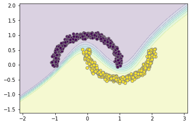
📈 L1 Q1: Build a Linear Model

Build and train a linear classification model using keras tf. Verify that the model is linear by either showing the weights or plotting the decision boundary (hint: you can use plot_boundaries above).

# Code Cell for L1 Q1
from tensorflow import keras
from tensorflow.keras import layers

model = keras.Sequential([
    #### YOUR CODE HERE ###
])

model.compile(
    optimizer='adam',
    loss='binary_crossentropy',
    metrics=['binary_accuracy'],
)

history = model.fit(X,y,
          batch_size=100,
          epochs=500,
          verbose=0)

model.summary()

results = pd.DataFrame(history.history)
display(results.tail())

y_pred = model.predict(X) > 0.5
px.scatter(x=X[:,0],y=X[:,1], color=y_pred.astype(str))

Model: "sequential_14"
_________________________________________________________________
Layer (type)                 Output Shape              Param #   
=================================================================
dense_51 (Dense)             (None, 2)                 6         
_________________________________________________________________
dense_52 (Dense)             (None, 2)                 6         
_________________________________________________________________
dense_53 (Dense)             (None, 2)                 6         
_________________________________________________________________
dense_54 (Dense)             (None, 1)                 3         
=================================================================
Total params: 21
Trainable params: 21
Non-trainable params: 0
_________________________________________________________________

	loss	binary_accuracy
495	0.225831	0.888
496	0.225785	0.887
497	0.226102	0.888
498	0.225775	0.886
499	0.225990	0.888

plot_boundaries(X, model)

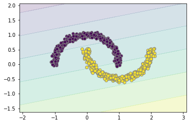
🌀 L1 Q2: Build a Non-Linear Model

Now add an activation function to your previous model. Does the model become non-linear?

# Code Cell for L1 Q2

model = keras.Sequential([
    #### YOUR CODE HERE ###
])

model.compile(
    optimizer='adam',
    loss='binary_crossentropy',
    metrics=['binary_accuracy'],
)

history = model.fit(X,y,
          batch_size=100,
          epochs=500,
          verbose=0)

results = pd.DataFrame(history.history)

display(results.tail())

y_pred = model.predict(X) > 0.5
px.scatter(x=X[:,0],y=X[:,1],color=y_pred.astype(str))

	loss	binary_accuracy
495	0.093515	0.981
496	0.092895	0.981
497	0.091976	0.982
498	0.091197	0.982
499	0.090521	0.982

plot_boundaries(X, model)

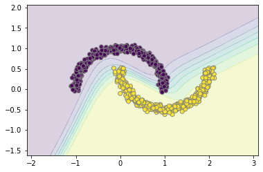
✨ L1 Q3: Add Complexity

Continue to add complexity to your Q3 model until you get an accuracy above 99%

# Code Cell for L1 Q3

model = keras.Sequential([
    #### YOUR CODE HERE ###
])

model.compile(
    optimizer='adam',
    loss='binary_crossentropy',
    metrics=['binary_accuracy'],
)

history = model.fit(X,y,
          batch_size=100,
          epochs=100,
          verbose=0)

results = pd.DataFrame(history.history)

display(results.tail())

y_pred = model.predict(X) > 0.5
px.scatter(x=X[:,0],y=X[:,1],color=y_pred.astype(str))

	loss	binary_accuracy
95	0.021280	1.0
96	0.019798	1.0
97	0.018461	1.0
98	0.017353	1.0
99	0.016389	1.0

plot_boundaries(X, model)