![]()
Python Foundations, Session 5: Pandas
Instructor: Wesley Beckner
Contact: wesleybeckner@gmail.com
Recording: Video (56 min)
special thanks to David Beck for their contribution to this material
Today, we will jump into the Pandas package. Packages are collections of related functions. These are the things we import. Pandas operates around a two dimensional data structure called a DataFrame, much like a spreadsheet in Excel. We will be importing our first dataset and viewing it, with Pandas!
5.1 Pandas
5.1.1 Pandas and Scikit-Learn load_datasets
We begin by loading the Pandas package. Packages are collections of functions that share a common utility. We've seen import before. Let's use it to import Pandas and all the richness that Pandas has.
We'll also use a very useful feature of the scikit-learn toolkit, the load_datasets module. We will do some very rudimentary tasks with this dataset, just to demonstrate the utility of load_datasets, then we will switch over to a more relevant dataset for our purposes.
import pandas
from sklearn.datasets import load_wine
import pandas
from sklearn.datasets import load_wine
We import a function load_wine that loads a simple data set we can play with called the Wine recognition dataset from the 1980s.
You can read more about that dataset here
dataset = load_wine()
print(dataset.DESCR)
dataset = load_wine()
print(dataset.DESCR)
.. _wine_dataset:

Wine recognition dataset
------------------------

**Data Set Characteristics:**

    :Number of Instances: 178 (50 in each of three classes)
    :Number of Attributes: 13 numeric, predictive attributes and the class
    :Attribute Information:
        - Alcohol
        - Malic acid
        - Ash
        - Alcalinity of ash
        - Magnesium
        - Total phenols
        - Flavanoids
        - Nonflavanoid phenols
        - Proanthocyanins
        - Color intensity
        - Hue
        - OD280/OD315 of diluted wines
        - Proline

    - class:
            - class_0
            - class_1
            - class_2

    :Summary Statistics:

    ============================= ==== ===== ======= =====
                                   Min   Max   Mean     SD
    ============================= ==== ===== ======= =====
    Alcohol:                      11.0  14.8    13.0   0.8
    Malic Acid:                   0.74  5.80    2.34  1.12
    Ash:                          1.36  3.23    2.36  0.27
    Alcalinity of Ash:            10.6  30.0    19.5   3.3
    Magnesium:                    70.0 162.0    99.7  14.3
    Total Phenols:                0.98  3.88    2.29  0.63
    Flavanoids:                   0.34  5.08    2.03  1.00
    Nonflavanoid Phenols:         0.13  0.66    0.36  0.12
    Proanthocyanins:              0.41  3.58    1.59  0.57
    Colour Intensity:              1.3  13.0     5.1   2.3
    Hue:                          0.48  1.71    0.96  0.23
    OD280/OD315 of diluted wines: 1.27  4.00    2.61  0.71
    Proline:                       278  1680     746   315
    ============================= ==== ===== ======= =====

    :Missing Attribute Values: None
    :Class Distribution: class_0 (59), class_1 (71), class_2 (48)
    :Creator: R.A. Fisher
    :Donor: Michael Marshall (MARSHALL%PLU@io.arc.nasa.gov)
    :Date: July, 1988

This is a copy of UCI ML Wine recognition datasets.
https://archive.ics.uci.edu/ml/machine-learning-databases/wine/wine.data

The data is the results of a chemical analysis of wines grown in the same
region in Italy by three different cultivators. There are thirteen different
measurements taken for different constituents found in the three types of
wine.

Original Owners:

Forina, M. et al, PARVUS -
An Extendible Package for Data Exploration, Classification and Correlation.
Institute of Pharmaceutical and Food Analysis and Technologies,
Via Brigata Salerno, 16147 Genoa, Italy.

Citation:

Lichman, M. (2013). UCI Machine Learning Repository
[https://archive.ics.uci.edu/ml]. Irvine, CA: University of California,
School of Information and Computer Science.

.. topic:: References

  (1) S. Aeberhard, D. Coomans and O. de Vel,
  Comparison of Classifiers in High Dimensional Settings,
  Tech. Rep. no. 92-02, (1992), Dept. of Computer Science and Dept. of
  Mathematics and Statistics, James Cook University of North Queensland.
  (Also submitted to Technometrics).

  The data was used with many others for comparing various
  classifiers. The classes are separable, though only RDA
  has achieved 100% correct classification.
  (RDA : 100%, QDA 99.4%, LDA 98.9%, 1NN 96.1% (z-transformed data))
  (All results using the leave-one-out technique)

  (2) S. Aeberhard, D. Coomans and O. de Vel,
  "THE CLASSIFICATION PERFORMANCE OF RDA"
  Tech. Rep. no. 92-01, (1992), Dept. of Computer Science and Dept. of
  Mathematics and Statistics, James Cook University of North Queensland.
  (Also submitted to Journal of Chemometrics).
df = pandas.DataFrame()
df = pandas.DataFrame()
5.1.1.1 import ... as ... pattern
Because we'll use it so much, we often import under a shortened name using the import ... as ... pattern:
import pandas as pd
import pandas as pd
5.1.2 Creating pandas DataFrames
DataFrames are two-dimensional tables of data that are the common data object we work with in Pandas. You can think of it as like an Excel spreadsheet.
Let's create an empty DataFrame and put the result into a variable called df. This is a popular choice for a DataFrame variable name.
df = pd.DataFrame()
df = pd.DataFrame()
Let's open the Wine dataset as a pandas DataFrame. Notice we change the value of the df variable to point to a new DataFrame.
df = pd.DataFrame(dataset.data, columns=dataset.feature_names)
df = pd.DataFrame(dataset.data, columns=dataset.feature_names)
5.1.2.1 From excel and csv
We will now be reading the data from this link. This is what we call a csv or comma separated value file. We have a method to read these directly into pandas:
df = pd.read_csv('https://raw.githubusercontent.com/wesleybeckner/technology_explorers/main/assets/imdb_movies.csv')
C:\Users\WesleyBeckner\AppData\Local\Temp\ipykernel_17180\2664770703.py:1: DtypeWarning: Columns (3) have mixed types. Specify dtype option on import or set low_memory=False.
  df = pd.read_csv('https://raw.githubusercontent.com/wesleybeckner/technology_explorers/main/assets/imdb_movies.csv')
We can do this in a similar way with excel files.
pd.read_excel('https://raw.githubusercontent.com/wesleybeckner/ds_for_engineers/main/data/truffle_margin/margin_data.xlsx')
| Base Cake | Truffle Type | Primary Flavor | Secondary Flavor | Color Group | Width | Height | Net Sales Quantity in KG | EBITDA | Product | |
|---|---|---|---|---|---|---|---|---|---|---|
| 0 | Tiramisu | Chocolate Outer | Doughnut | Egg Nog | Amethyst | 340 | 50 | 8244.500 | 21833.99 | Tiramisu-Chocolate Outer-Doughnut-Egg Nog-Amet... |
| 1 | Tiramisu | Chocolate Outer | Doughnut | Egg Nog | Amethyst | 1340 | 25 | 1857.000 | 21589.48 | Tiramisu-Chocolate Outer-Doughnut-Egg Nog-Amet... |
| 2 | Tiramisu | Chocolate Outer | Chocolate | Pear | Amethyst | 310 | 140 | 17365.000 | 19050.69 | Tiramisu-Chocolate Outer-Chocolate-Pear-Amethy... |
| 3 | Tiramisu | Chocolate Outer | Doughnut | Egg Nog | Amethyst | 449 | 50 | 14309.000 | 18573.01 | Tiramisu-Chocolate Outer-Doughnut-Egg Nog-Amet... |
| 4 | Tiramisu | Chocolate Outer | Doughnut | Rock and Rye | Amethyst | 640 | 80 | 25584.500 | 14790.90 | Tiramisu-Chocolate Outer-Doughnut-Rock and Rye... |
| ... | ... | ... | ... | ... | ... | ... | ... | ... | ... | ... |
| 2501 | Butter | Chocolate Outer | Lemon Bar | Wild Cherry Cream | Amethyst | 930 | 50 | 150352.000 | -97839.16 | Butter-Chocolate Outer-Lemon Bar-Wild Cherry C... |
| 2502 | Butter | Chocolate Outer | Cream Soda | Peppermint | Amethyst | 900 | 50 | 120451.400 | -98661.97 | Butter-Chocolate Outer-Cream Soda-Peppermint-A... |
| 2503 | Butter | Jelly Filled | Orange | Cucumber | Burgundy | 905 | 50 | 143428.580 | -122236.96 | Butter-Jelly Filled-Orange-Cucumber-Burgundy-9... |
| 2504 | Butter | Chocolate Outer | Horchata | Dill Pickle | Amethyst | 597 | 45 | 271495.572 | -128504.49 | Butter-Chocolate Outer-Horchata-Dill Pickle-Am... |
| 2505 | Butter | Candy Outer | Ginger Lime | Vanilla | Amethyst | 580 | 50 | 170567.065 | -137897.08 | Butter-Candy Outer-Ginger Lime-Vanilla-Amethys... |
2506 rows × 10 columns
5.1.2.2 from lists
my_list = [[1, 2, 3], [3, 4, 5], [5, 6, 7], [7, 8, 9]]
pd.DataFrame(my_list)
| 0 | 1 | 2 | |
|---|---|---|---|
| 0 | 1 | 2 | 3 |
| 1 | 3 | 4 | 5 |
| 2 | 5 | 6 | 7 |
| 3 | 7 | 8 | 9 |
pd.DataFrame([[1, 2, 3], [3, 4, 5], [5, 6, 7], [7, 8, 9]],
                   index=['a', 'b', 'c', 'd'], columns=['x', 'y', 'z'])
| x | y | z | |
|---|---|---|---|
| a | 1 | 2 | 3 |
| b | 3 | 4 | 5 |
| c | 5 | 6 | 7 |
| d | 7 | 8 | 9 |
5.1.2.3 from dictionaries
from_dict = pd.DataFrame({'A': ['apple', 'airplane'], 'B': ['bannana', 'bubbles']})
from_dict
| A | B | |
|---|---|---|
| 0 | apple | bannana |
| 1 | airplane | bubbles |
from_dict.to_dict()
{'A': {0: 'apple', 1: 'airplane'}, 'B': {0: 'bannana', 1: 'bubbles'}}
🏋️ Exercise 1: Create a DataFrame
Create a dictionary with the following keys: movies, songs, books. In each key list your top 5 favorites in the cooresponding category. Then use pd.DataFrame to turn this into a dictionary.
# Cell for Ex 1
5.1.2.4 on pandas.Series
pandas Series objects will percolate in our experience here and there, however they are not so important as for us to wish to spend dedicated time on them. For now, know that they are a lower-level data collection in the pandas framework. You can think of them as an individual column or row in the pandas dataframe. For more practice with these you can refer to this documentation
5.1.3 Viewing pandas dataframes
The head() and tail() methods show us the first and last rows of the data.
df.head()
df.tail()
df.head()
| imdb_title_id | title | original_title | year | date_published | genre | duration | country | language | director | writer | production_company | actors | description | avg_vote | votes | budget | usa_gross_income | worlwide_gross_income | metascore | reviews_from_users | reviews_from_critics | |
|---|---|---|---|---|---|---|---|---|---|---|---|---|---|---|---|---|---|---|---|---|---|---|
| 0 | tt0000009 | Miss Jerry | Miss Jerry | 1894 | 1894-10-09 | Romance | 45 | USA | None | Alexander Black | Alexander Black | Alexander Black Photoplays | Blanche Bayliss, William Courtenay, Chauncey D... | The adventures of a female reporter in the 1890s. | 5.9 | 154 | NaN | NaN | NaN | NaN | 1.0 | 2.0 |
| 1 | tt0000574 | The Story of the Kelly Gang | The Story of the Kelly Gang | 1906 | 1906-12-26 | Biography, Crime, Drama | 70 | Australia | None | Charles Tait | Charles Tait | J. and N. Tait | Elizabeth Tait, John Tait, Norman Campbell, Be... | True story of notorious Australian outlaw Ned ... | 6.1 | 589 | $ 2250 | NaN | NaN | NaN | 7.0 | 7.0 |
| 2 | tt0001892 | Den sorte drøm | Den sorte drøm | 1911 | 1911-08-19 | Drama | 53 | Germany, Denmark | NaN | Urban Gad | Urban Gad, Gebhard Schätzler-Perasini | Fotorama | Asta Nielsen, Valdemar Psilander, Gunnar Helse... | Two men of high rank are both wooing the beaut... | 5.8 | 188 | NaN | NaN | NaN | NaN | 5.0 | 2.0 |
| 3 | tt0002101 | Cleopatra | Cleopatra | 1912 | 1912-11-13 | Drama, History | 100 | USA | English | Charles L. Gaskill | Victorien Sardou | Helen Gardner Picture Players | Helen Gardner, Pearl Sindelar, Miss Fielding, ... | The fabled queen of Egypt's affair with Roman ... | 5.2 | 446 | $ 45000 | NaN | NaN | NaN | 25.0 | 3.0 |
| 4 | tt0002130 | L'Inferno | L'Inferno | 1911 | 1911-03-06 | Adventure, Drama, Fantasy | 68 | Italy | Italian | Francesco Bertolini, Adolfo Padovan | Dante Alighieri | Milano Film | Salvatore Papa, Arturo Pirovano, Giuseppe de L... | Loosely adapted from Dante's Divine Comedy and... | 7.0 | 2237 | NaN | NaN | NaN | NaN | 31.0 | 14.0 |
df.tail()
| imdb_title_id | title | original_title | year | date_published | genre | duration | country | language | director | writer | production_company | actors | description | avg_vote | votes | budget | usa_gross_income | worlwide_gross_income | metascore | reviews_from_users | reviews_from_critics | |
|---|---|---|---|---|---|---|---|---|---|---|---|---|---|---|---|---|---|---|---|---|---|---|
| 85850 | tt9908390 | Le lion | Le lion | 2020 | 2020-01-29 | Comedy | 95 | France, Belgium | French | Ludovic Colbeau-Justin | Alexandre Coquelle, Matthieu Le Naour | Monkey Pack Films | Dany Boon, Philippe Katerine, Anne Serra, Samu... | A psychiatric hospital patient pretends to be ... | 5.3 | 398 | NaN | NaN | $ 3507171 | NaN | NaN | 4.0 |
| 85851 | tt9911196 | De Beentjes van Sint-Hildegard | De Beentjes van Sint-Hildegard | 2020 | 2020-02-13 | Comedy, Drama | 103 | Netherlands | German, Dutch | Johan Nijenhuis | Radek Bajgar, Herman Finkers | Johan Nijenhuis & Co | Herman Finkers, Johanna ter Steege, Leonie ter... | A middle-aged veterinary surgeon believes his ... | 7.7 | 724 | NaN | NaN | $ 7299062 | NaN | 6.0 | 4.0 |
| 85852 | tt9911774 | Padmavyuhathile Abhimanyu | Padmavyuhathile Abhimanyu | 2019 | 2019-03-08 | Drama | 130 | India | Malayalam | Vineesh Aaradya | Vineesh Aaradya, Vineesh Aaradya | RMCC Productions | Anoop Chandran, Indrans, Sona Nair, Simon Brit... | NaN | 7.9 | 265 | NaN | NaN | NaN | NaN | NaN | NaN |
| 85853 | tt9914286 | Sokagin Çocuklari | Sokagin Çocuklari | 2019 | 2019-03-15 | Drama, Family | 98 | Turkey | Turkish | Ahmet Faik Akinci | Ahmet Faik Akinci, Kasim Uçkan | Gizem Ajans | Ahmet Faik Akinci, Belma Mamati, Metin Keçeci,... | NaN | 6.4 | 194 | NaN | NaN | $ 2833 | NaN | NaN | NaN |
| 85854 | tt9914942 | La vida sense la Sara Amat | La vida sense la Sara Amat | 2019 | 2020-02-05 | Drama | 74 | Spain | Catalan | Laura Jou | Coral Cruz, Pep Puig | La Xarxa de Comunicació Local | Maria Morera Colomer, Biel Rossell Pelfort, Is... | Pep, a 13-year-old boy, is in love with a girl... | 6.7 | 102 | NaN | NaN | $ 59794 | NaN | NaN | 2.0 |
The shape attribute shows us the number of elements:
df.shape
Note it doesn't have the () because it isn't a function - it is an attribute or variable attached to the df object.
df.shape
(85855, 22)
The columns attribute gives us the column names
df.columns
df.columns
Index(['imdb_title_id', 'title', 'original_title', 'year', 'date_published',
       'genre', 'duration', 'country', 'language', 'director', 'writer',
       'production_company', 'actors', 'description', 'avg_vote', 'votes',
       'budget', 'usa_gross_income', 'worlwide_gross_income', 'metascore',
       'reviews_from_users', 'reviews_from_critics'],
      dtype='object')
The index attribute gives us the index names
df.index
df.index
RangeIndex(start=0, stop=85855, step=1)
The dtypes attribute gives the data types of each column, remember the data type floating point*?:
df.dtypes
df.dtypes
imdb_title_id             object
title                     object
original_title            object
year                      object
date_published            object
genre                     object
duration                   int64
country                   object
language                  object
director                  object
writer                    object
production_company        object
actors                    object
description               object
avg_vote                 float64
votes                      int64
budget                    object
usa_gross_income          object
worlwide_gross_income     object
metascore                float64
reviews_from_users       float64
reviews_from_critics     float64
dtype: object
df.describe()
| duration | avg_vote | votes | metascore | reviews_from_users | reviews_from_critics | |
|---|---|---|---|---|---|---|
| count | 85855.000000 | 85855.000000 | 8.585500e+04 | 13305.000000 | 78258.000000 | 74058.000000 |
| mean | 100.351418 | 5.898656 | 9.493490e+03 | 55.896881 | 46.040826 | 27.479989 |
| std | 22.553848 | 1.234987 | 5.357436e+04 | 17.784874 | 178.511411 | 58.339158 |
| min | 41.000000 | 1.000000 | 9.900000e+01 | 1.000000 | 1.000000 | 1.000000 |
| 25% | 88.000000 | 5.200000 | 2.050000e+02 | 43.000000 | 4.000000 | 3.000000 |
| 50% | 96.000000 | 6.100000 | 4.840000e+02 | 57.000000 | 9.000000 | 8.000000 |
| 75% | 108.000000 | 6.800000 | 1.766500e+03 | 69.000000 | 27.000000 | 23.000000 |
| max | 808.000000 | 9.900000 | 2.278845e+06 | 100.000000 | 10472.000000 | 999.000000 |
🏋️ Exercise 2: Viewing DataFrames
Using the dataframe you made in exercise 1, return the following attributes: the datatype stored in each column, the column names, the indices, and the shape.
# Cell for Ex 2
5.1.4 Manipulating data with pandas
Here we'll cover some key features of manipulating data with pandas
5.1.4.1 Selection
Access columns by name using square-bracket indexing:
df['duration']
df['duration']
0         45
1         70
2         53
3        100
4         68
        ...
85850     95
85851    103
85852    130
85853     98
85854     74
Name: duration, Length: 85855, dtype: int64
Mathematical operations on columns happen element-wise:
df['duration'] / 60
df['duration'] / 60
0        0.750000
1        1.166667
2        0.883333
3        1.666667
4        1.133333
           ...
85850    1.583333
85851    1.716667
85852    2.166667
85853    1.633333
85854    1.233333
Name: duration, Length: 85855, dtype: float64
Columns can be created (or overwritten) with the assignment operator. Let's create a column with duration in hours.
df['duration (hours)'] = df['duration'] / 60
df['duration (hours)'] = df['duration'] / 60
Let's use the .head() function to see our new data!
df.head()
df.head()
| imdb_title_id | title | original_title | year | date_published | genre | duration | country | language | director | writer | production_company | actors | description | avg_vote | votes | budget | usa_gross_income | worlwide_gross_income | metascore | reviews_from_users | reviews_from_critics | duration (hours) | |
|---|---|---|---|---|---|---|---|---|---|---|---|---|---|---|---|---|---|---|---|---|---|---|---|
| 0 | tt0000009 | Miss Jerry | Miss Jerry | 1894 | 1894-10-09 | Romance | 45 | USA | None | Alexander Black | Alexander Black | Alexander Black Photoplays | Blanche Bayliss, William Courtenay, Chauncey D... | The adventures of a female reporter in the 1890s. | 5.9 | 154 | NaN | NaN | NaN | NaN | 1.0 | 2.0 | 0.750000 |
| 1 | tt0000574 | The Story of the Kelly Gang | The Story of the Kelly Gang | 1906 | 1906-12-26 | Biography, Crime, Drama | 70 | Australia | None | Charles Tait | Charles Tait | J. and N. Tait | Elizabeth Tait, John Tait, Norman Campbell, Be... | True story of notorious Australian outlaw Ned ... | 6.1 | 589 | $ 2250 | NaN | NaN | NaN | 7.0 | 7.0 | 1.166667 |
| 2 | tt0001892 | Den sorte drøm | Den sorte drøm | 1911 | 1911-08-19 | Drama | 53 | Germany, Denmark | NaN | Urban Gad | Urban Gad, Gebhard Schätzler-Perasini | Fotorama | Asta Nielsen, Valdemar Psilander, Gunnar Helse... | Two men of high rank are both wooing the beaut... | 5.8 | 188 | NaN | NaN | NaN | NaN | 5.0 | 2.0 | 0.883333 |
| 3 | tt0002101 | Cleopatra | Cleopatra | 1912 | 1912-11-13 | Drama, History | 100 | USA | English | Charles L. Gaskill | Victorien Sardou | Helen Gardner Picture Players | Helen Gardner, Pearl Sindelar, Miss Fielding, ... | The fabled queen of Egypt's affair with Roman ... | 5.2 | 446 | $ 45000 | NaN | NaN | NaN | 25.0 | 3.0 | 1.666667 |
| 4 | tt0002130 | L'Inferno | L'Inferno | 1911 | 1911-03-06 | Adventure, Drama, Fantasy | 68 | Italy | Italian | Francesco Bertolini, Adolfo Padovan | Dante Alighieri | Milano Film | Salvatore Papa, Arturo Pirovano, Giuseppe de L... | Loosely adapted from Dante's Divine Comedy and... | 7.0 | 2237 | NaN | NaN | NaN | NaN | 31.0 | 14.0 | 1.133333 |
5.1.4.1.1 loc and iloc
Pandas provides a powerful way to work with both rows and columns together, optionally using their label indices or numeric indices.
-
.loc :
Purely label-location based indexer for selection by label (but may also be used with a boolean array).
Important: If you use slicing in loc, it will return the end index as well -
.iloc:
Purely integer-location based indexing for selection by position (but may also be used with a boolean array).
df.columns[1]
'title'
df.loc[:5:2, [df.columns[1]]]
| title | |
|---|---|
| 0 | Miss Jerry |
| 2 | Den sorte drøm |
| 4 | L'Inferno |
df.iloc[-5:, [3,5]]
| year | genre | |
|---|---|---|
| 85850 | 2020 | Comedy |
| 85851 | 2020 | Comedy, Drama |
| 85852 | 2019 | Drama |
| 85853 | 2019 | Drama, Family |
| 85854 | 2019 | Drama |
5.1.4.1.2 column vs index access
df['duration'][0:10]
0     45
1     70
2     53
3    100
4     68
5     60
6     85
7    120
8    120
9     55
Name: duration, dtype: int64
# df[0]['duration'] # will return an error
my_list = [[10, 20, 30]]*4
mydf = pd.DataFrame(my_list,
                    index=['a','b','c','d'],
                    columns=['alpha', 'beta', 'gamma'])
mydf
| alpha | beta | gamma | |
|---|---|---|---|
| a | 10 | 20 | 30 |
| b | 10 | 20 | 30 |
| c | 10 | 20 | 30 |
| d | 10 | 20 | 30 |
mydf.loc['a', 'alpha'] = 'mychange'
# using this you will get a setting
# with copy warning (depending on your pandas warning settings)
# mydf['alpha']['a'] = 'newchange'
You want to use loc or iloc when setting new values to pandas dataframes.
🏋️ Exercise 3: Selecting
select the first 10 rows of the country, genre, and year columns using loc. Repeat the same exercise using iloc
# Cell for Ex 3
5.1.4.2 Filtering
filtering down your selection will be BIGLY useful in your data quests
5.1.4.2.1 By String
one of the first tools we'll use to filter our dataset is the .str.contains method. Let's take an example.
# remember, if we don't remember our column mames we can quickly pull them up
# with:
df.columns
Index(['imdb_title_id', 'title', 'original_title', 'year', 'date_published',
       'genre', 'duration', 'country', 'language', 'director', 'writer',
       'production_company', 'actors', 'description', 'avg_vote', 'votes',
       'budget', 'usa_gross_income', 'worlwide_gross_income', 'metascore',
       'reviews_from_users', 'reviews_from_critics', 'duration (hours)'],
      dtype='object')
[df['description'].str.contains('a.i.', na=False)]
[0        False
 1         True
 2         True
 3        False
 4         True
          ...
 85850     True
 85851    False
 85852    False
 85853    False
 85854    False
 Name: description, Length: 85855, dtype: bool]
df.iloc[17920]['description']
'A scientist creates Proteus--an organic super computer with artificial intelligence which becomes obsessed with human beings, and in particular the creators wife.'
df[df['description'].str.contains('artificial intelligence', na=False)]
| imdb_title_id | title | original_title | year | date_published | genre | duration | country | language | director | writer | production_company | actors | description | avg_vote | votes | budget | usa_gross_income | worlwide_gross_income | metascore | reviews_from_users | reviews_from_critics | duration (hours) | |
|---|---|---|---|---|---|---|---|---|---|---|---|---|---|---|---|---|---|---|---|---|---|---|---|
| 17920 | tt0075931 | Generazione Proteus | Demon Seed | 1977 | 1977-12-31 | Horror, Sci-Fi | 94 | USA | English | Donald Cammell | Dean R. Koontz, Robert Jaffe | Metro-Goldwyn-Mayer (MGM) | Julie Christie, Fritz Weaver, Gerrit Graham, B... | A scientist creates Proteus--an organic super ... | 6.3 | 7994 | NaN | NaN | NaN | 55.0 | 71.0 | 81.0 | 1.566667 |
| 44484 | tt0382992 | Stealth - Arma suprema | Stealth | 2005 | 2005-09-02 | Action, Adventure, Sci-Fi | 121 | USA | English, Korean, Russian, Spanish | Rob Cohen | W.D. Richter | Columbia Pictures | Josh Lucas, Jessica Biel, Jamie Foxx, Sam Shep... | Deeply ensconced in a top-secret military prog... | 5.1 | 51365 | $ 135000000 | $ 32116746 | $ 79268322 | 35.0 | 401.0 | 150.0 | 2.016667 |
| 65411 | tt2209764 | Transcendence | Transcendence | 2014 | 2014-04-17 | Action, Drama, Sci-Fi | 119 | UK, China, USA | English | Wally Pfister | Jack Paglen | Alcon Entertainment | Johnny Depp, Rebecca Hall, Paul Bettany, Cilli... | A scientist's drive for artificial intelligenc... | 6.3 | 213720 | $ 100000000 | $ 23022309 | $ 103039258 | 42.0 | 554.0 | 373.0 | 1.983333 |
| 68589 | tt2769184 | Debug | Debug | 2014 | 2015-02-07 | Horror, Sci-Fi | 86 | Canada | English | David Hewlett | David Hewlett | Copperheart Entertainment | Tenika Davis, Jason Momoa, Adrian Holmes, Kjar... | Six young computer hackers, sent to work on a ... | 4.3 | 2244 | NaN | NaN | NaN | NaN | 38.0 | 30.0 | 1.433333 |
| 71500 | tt3502284 | Kikaidâ Reboot | Kikaidâ Reboot | 2014 | 2014-05-24 | Action | 110 | Japan | Japanese | Ten Shimoyama | Shôtarô Ishinomori, Kento Shimoyama | Asatsu-DK | Jingi Irie, Kazushige Nagashima, Aimi Satsukaw... | Komyoji Nobuhiko is a genius and leader in rob... | 5.6 | 110 | NaN | NaN | NaN | NaN | 2.0 | 2.0 | 1.833333 |
| 75759 | tt4788944 | Robot Sound | Robot Sound | 2016 | 2016-01-27 | Sci-Fi | 117 | South Korea | Korean, English | Ho-jae Lee | Soyoung Lee | NaN | Erik Brown, Soo-bin Chae, Dean Dawson, Lee Han... | The plot revolves around a robotic satellite w... | 6.9 | 191 | NaN | NaN | $ 2843718 | NaN | 3.0 | 4.0 | 1.950000 |
| 75907 | tt4839424 | Qi che ren zong dong yuan | Qi che ren zong dong yuan | 2015 | 2015-07-03 | Animation, Adventure, Family | 85 | China | Mandarin | Jianrong Zhuo | NaN | Xiamen Lanhuoyan Film Animation Co. | Christopher Petrosian, Dawei Hu, Xinxuan Liu, ... | The film revolves around a genius engineer who... | 1.1 | 121 | NaN | NaN | NaN | NaN | 2.0 | NaN | 1.416667 |
| 76214 | tt4937114 | Rogue Warrior: Robot Fighter | Rogue Warrior: Robot Fighter | 2016 | 2016-09-02 | Action, Sci-Fi | 101 | USA | English | Neil Johnson | Neil Johnson | Empire Motion pictures | Tracey Birdsall, William Kircher, Daz Crawford... | In the distant future, humanity is overthrown ... | 4.9 | 2574 | $ 3800000 | NaN | NaN | NaN | 22.0 | 26.0 | 1.683333 |
| 79921 | tt6197070 | Blood Machines | Blood Machines | 2019 | 2020-09-01 | Adventure, Music, Sci-Fi | 50 | France | English | Raphaël Hernandez, Seth Ickerman | Raphaël Hernandez, Seth Ickerman | Logical Pictures | Elisa Lasowski, Anders Heinrichsen, Christian ... | An artificial intelligence escapes her spacesh... | 6.1 | 2023 | NaN | NaN | NaN | NaN | 70.0 | 55.0 | 0.833333 |
| 83905 | tt8196068 | Twisted Pair | Twisted Pair | 2018 | 2018-10-03 | Drama, Fantasy, Sci-Fi | 89 | USA | English | Neil Breen | Neil Breen | Neil Breen Films | Neil Breen, Sara Meritt, Siohbon Chevy Ebrahim... | Identical twin brothers become hybrid A.I (art... | 5.9 | 1313 | $ 3 | NaN | NaN | NaN | 69.0 | 4.0 | 1.483333 |
| 84615 | tt8712750 | A.M.I. | A.M.I. | 2019 | 2019-07-02 | Horror, Thriller | 77 | Canada | English | Rusty Nixon | Rusty Nixon, Evan Tylor | 1160594 B.C. | Debs Howard, Philip Granger, Bonnie Hay, Sam R... | A seventeen year old girl forms a co-dependent... | 3.9 | 1399 | NaN | NaN | NaN | NaN | 91.0 | 13.0 | 1.283333 |
| 85361 | tt9308170 | Özgür Dünya | Özgür Dünya | 2019 | 2019-03-22 | Action, Adventure, Family | 122 | Turkey | Turkish | Faruk Aksoy, Sevki Es | Faruk Aksoy, Hüseyin Aksu | Ay Yapim | Murat Serezli, Rabia Soyturk, Gürbey Ileri, Ha... | The story of a game managed by artificial inte... | 2.3 | 340 | NaN | NaN | $ 50537 | NaN | 2.0 | NaN | 2.033333 |
or if you know the exact string you are looking for
df[df['title'] == "Fight Club"]
| imdb_title_id | title | original_title | year | date_published | genre | duration | country | language | director | writer | production_company | actors | description | avg_vote | votes | budget | usa_gross_income | worlwide_gross_income | metascore | reviews_from_users | reviews_from_critics | duration (hours) | |
|---|---|---|---|---|---|---|---|---|---|---|---|---|---|---|---|---|---|---|---|---|---|---|---|
| 32487 | tt0137523 | Fight Club | Fight Club | 1999 | 1999-10-29 | Drama | 139 | USA, Germany | English | David Fincher | Chuck Palahniuk, Jim Uhls | Fox 2000 Pictures | Edward Norton, Brad Pitt, Meat Loaf, Zach Gren... | An insomniac office worker and a devil-may-car... | 8.8 | 1807440 | $ 63000000 | $ 37030102 | $ 101218804 | 66.0 | 3758.0 | 370.0 | 2.316667 |
5.1.4.2.2 By numerical value
df[df['votes'] > 1000]
| imdb_title_id | title | original_title | year | date_published | genre | duration | country | language | director | writer | production_company | actors | description | avg_vote | votes | budget | usa_gross_income | worlwide_gross_income | metascore | reviews_from_users | reviews_from_critics | duration (hours) | |
|---|---|---|---|---|---|---|---|---|---|---|---|---|---|---|---|---|---|---|---|---|---|---|---|
| 4 | tt0002130 | L'Inferno | L'Inferno | 1911 | 1911-03-06 | Adventure, Drama, Fantasy | 68 | Italy | Italian | Francesco Bertolini, Adolfo Padovan | Dante Alighieri | Milano Film | Salvatore Papa, Arturo Pirovano, Giuseppe de L... | Loosely adapted from Dante's Divine Comedy and... | 7.0 | 2237 | NaN | NaN | NaN | NaN | 31.0 | 14.0 | 1.133333 |
| 11 | tt0002844 | Fantômas - À l'ombre de la guillotine | Fantômas - À l'ombre de la guillotine | 1913 | 1913-05-12 | Crime, Drama | 54 | France | French | Louis Feuillade | Marcel Allain, Louis Feuillade | Société des Etablissements L. Gaumont | René Navarre, Edmund Breon, Georges Melchior, ... | Inspector Juve is tasked to investigate and ca... | 7.0 | 1944 | NaN | NaN | NaN | NaN | 9.0 | 28.0 | 0.900000 |
| 13 | tt0003037 | Juve contre Fantômas | Juve contre Fantômas | 1913 | 1913-09-08 | Crime, Drama | 61 | France | French | Louis Feuillade | Marcel Allain, Louis Feuillade | Société des Etablissements L. Gaumont | René Navarre, Edmund Breon, Georges Melchior, ... | In Part Two of Louis Feuillade's 5 1/2-hour ep... | 7.0 | 1349 | NaN | NaN | NaN | NaN | 8.0 | 23.0 | 1.016667 |
| 16 | tt0003165 | Le mort qui tue | Le mort qui tue | 1913 | 1913-11-06 | Crime, Drama, Mystery | 90 | France | French | Louis Feuillade | Marcel Allain, Louis Feuillade | Société des Etablissements L. Gaumont | René Navarre, Edmund Breon, Georges Melchior, ... | After a body disappears from inside the prison... | 7.0 | 1050 | NaN | NaN | NaN | NaN | 6.0 | 18.0 | 1.500000 |
| 18 | tt0003419 | Lo studente di Praga | Der Student von Prag | 1913 | 1913-08-22 | Drama, Fantasy, Horror | 85 | Germany | German, English | Paul Wegener, Stellan Rye | Hanns Heinz Ewers, Hanns Heinz Ewers | Deutsche Bioscop GmbH | Paul Wegener, Grete Berger, Lyda Salmonova, Jo... | Balduin, a student of Prague, leaves his royst... | 6.5 | 1768 | NaN | NaN | NaN | NaN | 20.0 | 26.0 | 1.416667 |
| ... | ... | ... | ... | ... | ... | ... | ... | ... | ... | ... | ... | ... | ... | ... | ... | ... | ... | ... | ... | ... | ... | ... | ... |
| 85811 | tt9860728 | Falling Inn Love - Ristrutturazione con amore | Falling Inn Love | 2019 | 2019-08-29 | Comedy, Romance | 98 | USA | English | Roger Kumble | Elizabeth Hackett, Hilary Galanoy | NaN | Christina Milian, Adam Demos, Jeffrey Bowyer-C... | When city girl Gabriela spontaneously enters a... | 5.6 | 14108 | NaN | NaN | NaN | NaN | 265.0 | 32.0 | 1.633333 |
| 85817 | tt9866700 | Paranormal Investigation | Paranormal Investigation | 2018 | 2018-12-01 | Horror, Thriller | 92 | France | French | Franck Phelizon | NaN | Baril Pictures | Jose Atuncar, Claudine Bertin, Cedric Henquez,... | When a young man becomes possessed after playi... | 3.7 | 1299 | NaN | NaN | NaN | NaN | 334.0 | 11.0 | 1.533333 |
| 85837 | tt9894470 | VFW | VFW | 2019 | 2020-02-14 | Action, Crime, Horror | 92 | USA | English | Joe Begos | Max Brallier, Matthew McArdle | Fangoria | Stephen Lang, William Sadler, Fred Williamson,... | A group of old war veterans put their lives on... | 6.1 | 4178 | NaN | NaN | $ 23101 | 72.0 | 83.0 | 94.0 | 1.533333 |
| 85839 | tt9898858 | Coffee & Kareem | Coffee & Kareem | 2020 | 2020-04-03 | Action, Comedy | 88 | USA | English | Michael Dowse | Shane Mack | Pacific Electric Picture Company | Ed Helms, Taraji P. Henson, Terrence Little Ga... | Twelve-year-old Kareem Manning hires a crimina... | 5.1 | 10627 | NaN | NaN | NaN | 35.0 | 388.0 | 64.0 | 1.466667 |
| 85843 | tt9900782 | Kaithi | Kaithi | 2019 | 2019-10-25 | Action, Thriller | 145 | India | Tamil | Lokesh Kanagaraj | Lokesh Kanagaraj, Pon Parthiban | Dream Warrior Pictures | Karthi, Narain, Ramana, George Maryan, Harish ... | A recently released prisoner becomes involved ... | 8.5 | 8400 | INR 240000000 | NaN | $ 524061 | NaN | 188.0 | 8.0 | 2.416667 |
29362 rows × 23 columns
🏋️ Exercise 4: Filtering
- Filter
dffor all the movies that are longer than 2 hours - Filter
dffor all movies where 'day' is in the title
# Cell for Ex 4
5.1.4.3 Select, filter, operation
The real power of Pandas comes in its tools for grouping and aggregating data. Here we'll look at value counts and the basics of group-by operations.
# a basic select, filter, operate procedure would look like:
df[df['country'] == 'USA']['duration'].describe()
count    28511.000000
mean        93.050437
std         18.576873
min         42.000000
25%         84.000000
50%         91.000000
75%        100.000000
max        398.000000
Name: duration, dtype: float64
we can invert the selection with ~
df[~(df['country'] == 'USA')]['duration'].describe()
count    57344.000000
mean       103.981410
std         23.459158
min         41.000000
25%         90.000000
50%         99.000000
75%        112.000000
max        808.000000
Name: duration, dtype: float64
In preparation for grouping the data, let's bin the instances by their duration (we could have chosen any numerical column). For that, we'll use pd.cut. The documentation for pd.cut can be found here. It is used to bin values into discrete intervals. This is like a histogram where for each bin along the range of data values, you count the number of occurrences of that bin. in our example, we'll use 10 bins and let Pandas decide how to evenly divide the range into the bins. Let's see it in action.
df['duration_group'] = pd.cut(df['duration'], 10)
df.head()
df.dtypes
df['duration_group'] = pd.cut(df['duration'], 10)
df.head()
| imdb_title_id | title | original_title | year | date_published | genre | duration | country | language | director | writer | production_company | actors | description | avg_vote | votes | budget | usa_gross_income | worlwide_gross_income | metascore | reviews_from_users | reviews_from_critics | duration (hours) | duration_group | |
|---|---|---|---|---|---|---|---|---|---|---|---|---|---|---|---|---|---|---|---|---|---|---|---|---|
| 0 | tt0000009 | Miss Jerry | Miss Jerry | 1894 | 1894-10-09 | Romance | 45 | USA | None | Alexander Black | Alexander Black | Alexander Black Photoplays | Blanche Bayliss, William Courtenay, Chauncey D... | The adventures of a female reporter in the 1890s. | 5.9 | 154 | NaN | NaN | NaN | NaN | 1.0 | 2.0 | 0.750000 | (40.233, 117.7] |
| 1 | tt0000574 | The Story of the Kelly Gang | The Story of the Kelly Gang | 1906 | 1906-12-26 | Biography, Crime, Drama | 70 | Australia | None | Charles Tait | Charles Tait | J. and N. Tait | Elizabeth Tait, John Tait, Norman Campbell, Be... | True story of notorious Australian outlaw Ned ... | 6.1 | 589 | $ 2250 | NaN | NaN | NaN | 7.0 | 7.0 | 1.166667 | (40.233, 117.7] |
| 2 | tt0001892 | Den sorte drøm | Den sorte drøm | 1911 | 1911-08-19 | Drama | 53 | Germany, Denmark | NaN | Urban Gad | Urban Gad, Gebhard Schätzler-Perasini | Fotorama | Asta Nielsen, Valdemar Psilander, Gunnar Helse... | Two men of high rank are both wooing the beaut... | 5.8 | 188 | NaN | NaN | NaN | NaN | 5.0 | 2.0 | 0.883333 | (40.233, 117.7] |
| 3 | tt0002101 | Cleopatra | Cleopatra | 1912 | 1912-11-13 | Drama, History | 100 | USA | English | Charles L. Gaskill | Victorien Sardou | Helen Gardner Picture Players | Helen Gardner, Pearl Sindelar, Miss Fielding, ... | The fabled queen of Egypt's affair with Roman ... | 5.2 | 446 | $ 45000 | NaN | NaN | NaN | 25.0 | 3.0 | 1.666667 | (40.233, 117.7] |
| 4 | tt0002130 | L'Inferno | L'Inferno | 1911 | 1911-03-06 | Adventure, Drama, Fantasy | 68 | Italy | Italian | Francesco Bertolini, Adolfo Padovan | Dante Alighieri | Milano Film | Salvatore Papa, Arturo Pirovano, Giuseppe de L... | Loosely adapted from Dante's Divine Comedy and... | 7.0 | 2237 | NaN | NaN | NaN | NaN | 31.0 | 14.0 | 1.133333 | (40.233, 117.7] |
df.dtypes
imdb_title_id              object
title                      object
original_title             object
year                       object
date_published             object
genre                      object
duration                    int64
country                    object
language                   object
director                   object
writer                     object
production_company         object
actors                     object
description                object
avg_vote                  float64
votes                       int64
budget                     object
usa_gross_income           object
worlwide_gross_income      object
metascore                 float64
reviews_from_users        float64
reviews_from_critics      float64
duration (hours)          float64
duration_group           category
dtype: object
Pandas includes an array of useful functionality for manipulating and analyzing tabular data. We'll take a look at two of these here.
The pandas.value_counts returns statistics on the unique values within each column.
We can use it, for example, to break down the movies by their duration group that we just created:
pd.value_counts(df['duration_group'], sort=False)
pd.value_counts(df['duration_group'], sort=False)
(40.233, 117.7]    72368
(117.7, 194.4]     13197
(194.4, 271.1]       228
(271.1, 347.8]        40
(347.8, 424.5]        11
(424.5, 501.2]         4
(501.2, 577.9]         4
(577.9, 654.6]         1
(654.6, 731.3]         1
(731.3, 808.0]         1
Name: duration_group, dtype: int64
What happens if we try this on a continuous valued variable?
pd.value_counts(df['duration'])
pd.value_counts(df['duration'])
90     5162
95     3194
100    3106
92     2418
93     2414
       ...
279       1
301       1
345       1
729       1
319       1
Name: duration, Length: 266, dtype: int64
🏋️ Exercise 5: value_counts, unique, nunique
We can do a little data exploration with this by seeing how common different values are. Play around with these pandas methods:
value_counts()unique()nunique()
Also be sure to use:
- selection
- filteration
- (and you are already using operation with the above mentioned pandas methods, value_counts, unique, nunique (: )
Do so with 3 different columns in the dataframe
# Cell for Exercise 5
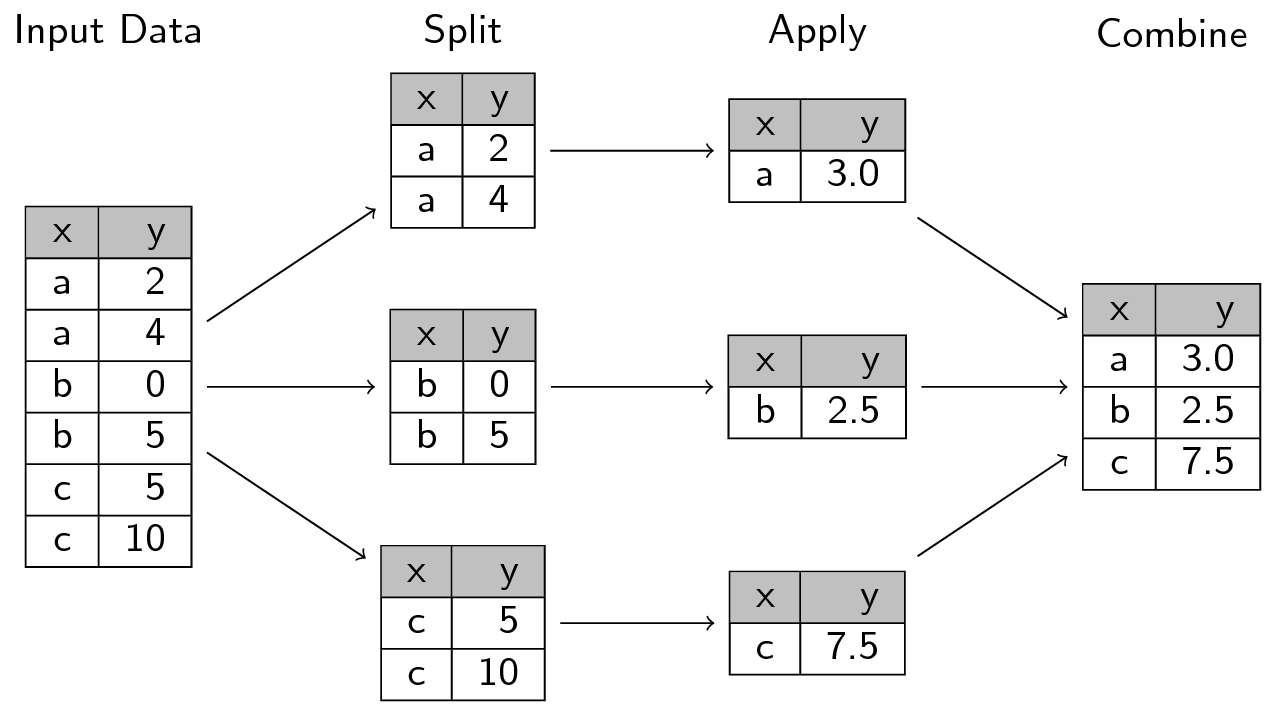
5.1.4.4 Group-by Operation
One of the killer features of the Pandas dataframe is the ability to do group-by operations. You can visualize the group-by like this (image borrowed from the Python Data Science Handbook)
5.1.4.5 Summary statistics with groupby: value_counts, count, describe
Let's break take this in smaller steps.
Recall our duration_group column.
pd.value_counts(df['duration_group'])
pd.value_counts(df['duration_group'])
(40.233, 117.7]    72368
(117.7, 194.4]     13197
(194.4, 271.1]       228
(271.1, 347.8]        40
(347.8, 424.5]        11
(501.2, 577.9]         4
(424.5, 501.2]         4
(731.3, 808.0]         1
(654.6, 731.3]         1
(577.9, 654.6]         1
Name: duration_group, dtype: int64
groupby allows us to look at the number of values for each column and each value. The group by documentation is here. Basically, groupby allows us to create groups of records based on their values. Let's count how many records, or rows, in our data set fall into each bin of our duration data.
df.groupby(['duration_group']).count()
df.groupby(['duration_group']).count()
| imdb_title_id | title | original_title | year | date_published | genre | duration | country | language | director | writer | production_company | actors | description | avg_vote | votes | budget | usa_gross_income | worlwide_gross_income | metascore | reviews_from_users | reviews_from_critics | duration (hours) | |
|---|---|---|---|---|---|---|---|---|---|---|---|---|---|---|---|---|---|---|---|---|---|---|---|
| duration_group | |||||||||||||||||||||||
| (40.233, 117.7] | 72368 | 72368 | 72368 | 72368 | 72368 | 72368 | 72368 | 72315 | 71618 | 72309 | 71474 | 68922 | 72304 | 70464 | 72368 | 72368 | 19493 | 12123 | 24645 | 10759 | 65972 | 63321 | 72368 |
| (117.7, 194.4] | 13197 | 13197 | 13197 | 13197 | 13197 | 13197 | 13197 | 13186 | 13122 | 13171 | 12528 | 12211 | 13192 | 12990 | 13197 | 13197 | 4133 | 3153 | 6298 | 2506 | 12017 | 10493 | 13197 |
| (194.4, 271.1] | 228 | 228 | 228 | 228 | 228 | 228 | 228 | 228 | 221 | 226 | 221 | 207 | 228 | 226 | 228 | 228 | 70 | 40 | 59 | 28 | 215 | 188 | 228 |
| (271.1, 347.8] | 40 | 40 | 40 | 40 | 40 | 40 | 40 | 40 | 40 | 40 | 39 | 39 | 40 | 38 | 40 | 40 | 10 | 5 | 9 | 8 | 37 | 37 | 40 |
| (347.8, 424.5] | 11 | 11 | 11 | 11 | 11 | 11 | 11 | 11 | 10 | 11 | 11 | 10 | 11 | 11 | 11 | 11 | 1 | 3 | 3 | 1 | 9 | 10 | 11 |
| (424.5, 501.2] | 4 | 4 | 4 | 4 | 4 | 4 | 4 | 4 | 4 | 4 | 4 | 4 | 4 | 4 | 4 | 4 | 1 | 0 | 0 | 1 | 4 | 4 | 4 |
| (501.2, 577.9] | 4 | 4 | 4 | 4 | 4 | 4 | 4 | 4 | 4 | 4 | 4 | 4 | 4 | 4 | 4 | 4 | 1 | 0 | 0 | 0 | 2 | 3 | 4 |
| (577.9, 654.6] | 1 | 1 | 1 | 1 | 1 | 1 | 1 | 1 | 1 | 1 | 1 | 1 | 1 | 1 | 1 | 1 | 1 | 0 | 0 | 0 | 0 | 0 | 1 |
| (654.6, 731.3] | 1 | 1 | 1 | 1 | 1 | 1 | 1 | 1 | 1 | 1 | 0 | 1 | 1 | 1 | 1 | 1 | 0 | 1 | 1 | 1 | 1 | 1 | 1 |
| (731.3, 808.0] | 1 | 1 | 1 | 1 | 1 | 1 | 1 | 1 | 1 | 1 | 1 | 1 | 1 | 1 | 1 | 1 | 0 | 1 | 1 | 1 | 1 | 1 | 1 |
Now, let's find the mean of each of the columns for each duration_group. Notice what happens to the non-numeric columns.
df.groupby(['duration_group']).mean()
df.groupby(['duration_group']).mean()
| duration | avg_vote | votes | metascore | reviews_from_users | reviews_from_critics | duration (hours) | |
|---|---|---|---|---|---|---|---|
| duration_group | |||||||
| (40.233, 117.7] | 93.147026 | 5.786671 | 6604.507932 | 54.153267 | 35.944037 | 24.517601 | 1.552450 |
| (117.7, 194.4] | 136.552550 | 6.488513 | 25010.089414 | 63.042298 | 100.725639 | 45.365958 | 2.275876 |
| (194.4, 271.1] | 220.394737 | 6.997368 | 30003.302632 | 76.500000 | 94.711628 | 29.015957 | 3.673246 |
| (271.1, 347.8] | 302.975000 | 6.810000 | 4201.275000 | 79.375000 | 19.378378 | 21.513514 | 5.049583 |
| (347.8, 424.5] | 384.636364 | 7.181818 | 2602.545455 | 89.000000 | 18.333333 | 18.100000 | 6.410606 |
| (424.5, 501.2] | 454.000000 | 7.700000 | 2589.000000 | 59.000000 | 19.250000 | 24.500000 | 7.566667 |
| (501.2, 577.9] | 547.500000 | 7.875000 | 206.500000 | NaN | 1.500000 | 8.666667 | 9.125000 |
| (577.9, 654.6] | 580.000000 | 5.800000 | 157.000000 | NaN | NaN | NaN | 9.666667 |
| (654.6, 731.3] | 729.000000 | 7.800000 | 1126.000000 | 87.000000 | 13.000000 | 30.000000 | 12.150000 |
| (731.3, 808.0] | 808.000000 | 7.700000 | 473.000000 | 77.000000 | 5.000000 | 23.000000 | 13.466667 |
You can specify a groupby using the names of table columns and compute other functions, such as the sum, count, std, and describe.
df.groupby(['duration_group'])['metascore'].describe()
df.groupby(['duration_group'])['metascore'].describe()
| count | mean | std | min | 25% | 50% | 75% | max | |
|---|---|---|---|---|---|---|---|---|
| duration_group | ||||||||
| (40.233, 117.7] | 10759.0 | 54.153267 | 17.655622 | 1.0 | 41.00 | 55.0 | 67.00 | 100.0 |
| (117.7, 194.4] | 2506.0 | 63.042298 | 16.265137 | 9.0 | 52.00 | 64.0 | 75.00 | 100.0 |
| (194.4, 271.1] | 28.0 | 76.500000 | 20.532720 | 10.0 | 69.75 | 82.0 | 90.00 | 100.0 |
| (271.1, 347.8] | 8.0 | 79.375000 | 12.070478 | 56.0 | 72.25 | 84.5 | 88.25 | 90.0 |
| (347.8, 424.5] | 1.0 | 89.000000 | NaN | 89.0 | 89.00 | 89.0 | 89.00 | 89.0 |
| (424.5, 501.2] | 1.0 | 59.000000 | NaN | 59.0 | 59.00 | 59.0 | 59.00 | 59.0 |
| (501.2, 577.9] | 0.0 | NaN | NaN | NaN | NaN | NaN | NaN | NaN |
| (577.9, 654.6] | 0.0 | NaN | NaN | NaN | NaN | NaN | NaN | NaN |
| (654.6, 731.3] | 1.0 | 87.000000 | NaN | 87.0 | 87.00 | 87.0 | 87.00 | 87.0 |
| (731.3, 808.0] | 1.0 | 77.000000 | NaN | 77.0 | 77.00 | 77.0 | 77.00 | 77.0 |
The simplest version of a groupby looks like this, and you can use almost any aggregation function you wish (mean, median, sum, minimum, maximum, standard deviation, count, etc.)
<data object>.groupby(<grouping values>).<aggregate>()
You can even group by multiple values: for example we can look at the metascore grouped by the duration_group and country.
df.groupby(['duration_group', 'country'])['metascore'].describe()
| count | mean | std | min | 25% | 50% | 75% | max | ||
|---|---|---|---|---|---|---|---|---|---|
| duration_group | country | ||||||||
| (40.233, 117.7] | Afghanistan, France | 0.0 | NaN | NaN | NaN | NaN | NaN | NaN | NaN |
| Afghanistan, France, Germany, UK | 1.0 | 64.0 | NaN | 64.0 | 64.0 | 64.0 | 64.0 | 64.0 | |
| Afghanistan, Iran | 0.0 | NaN | NaN | NaN | NaN | NaN | NaN | NaN | |
| Afghanistan, Ireland, Japan, Iran, Netherlands | 1.0 | 83.0 | NaN | 83.0 | 83.0 | 83.0 | 83.0 | 83.0 | |
| Albania | 0.0 | NaN | NaN | NaN | NaN | NaN | NaN | NaN | |
| ... | ... | ... | ... | ... | ... | ... | ... | ... | ... |
| (501.2, 577.9] | Philippines, Netherlands, Sweden | 0.0 | NaN | NaN | NaN | NaN | NaN | NaN | NaN |
| Russia | 0.0 | NaN | NaN | NaN | NaN | NaN | NaN | NaN | |
| (577.9, 654.6] | Soviet Union | 0.0 | NaN | NaN | NaN | NaN | NaN | NaN | NaN |
| (654.6, 731.3] | France | 1.0 | 87.0 | NaN | 87.0 | 87.0 | 87.0 | 87.0 | 87.0 |
| (731.3, 808.0] | Argentina | 1.0 | 77.0 | NaN | 77.0 | 77.0 | 77.0 | 77.0 | 77.0 |
5565 rows × 8 columns
🏋️ Exercise 6: Group-by
- use
pd.cutto perform a grouping of one or more of the dataframe columns - use
groupbyto group by that (those) columns and then perform - three different statistical summaries in three separate instances
# Cell for excercise 6