Data Science Foundations
Session 1: Regression and Analysis¶

Instructor: Wesley Beckner

In this session we will look at fitting data to a curve using regression. We will also look at using regression to make predictions for new data points by dividing our data into a training and a testing set. Finally we will examine how much error we make in our fit and then in our predictions by computing the mean squared error.

1.0 Preparing Environment and Importing Data¶

back to top

1.0.1 Import Packages¶

back to top

# Import pandas, pyplot, ipywidgets
import pandas as pd  
from matplotlib import pyplot as plt
from ipywidgets import interact

# Import Scikit-Learn library for the regression models
import sklearn         
from sklearn import linear_model
from sklearn.model_selection import train_test_split
from sklearn.metrics import mean_squared_error, r2_score

# for enrichment topics
import seaborn as sns
import numpy as np
import scipy

1.0.2 Load Dataset¶

back to top

For our discussion on regression and descriptive statistics today we will use a well known dataset of different wines and their quality ratings

df = pd.read_csv("https://raw.githubusercontent.com/wesleybeckner/"\
                 "ds_for_engineers/main/data/wine_quality/winequalityN.csv")
df.shape

(6497, 13)

df.head()

	type	fixed acidity	volatile acidity	citric acid	residual sugar	chlorides	free sulfur dioxide	total sulfur dioxide	density	pH	sulphates	alcohol	quality
0	white	7.0	0.27	0.36	20.7	0.045	45.0	170.0	1.0010	3.00	0.45	8.8	6
1	white	6.3	0.30	0.34	1.6	0.049	14.0	132.0	0.9940	3.30	0.49	9.5	6
2	white	8.1	0.28	0.40	6.9	0.050	30.0	97.0	0.9951	3.26	0.44	10.1	6
3	white	7.2	0.23	0.32	8.5	0.058	47.0	186.0	0.9956	3.19	0.40	9.9	6
4	white	7.2	0.23	0.32	8.5	0.058	47.0	186.0	0.9956	3.19	0.40	9.9	6

1.1 What is regression?¶

It is the process of finding a relationship between dependent and independent variables to find trends in data. This abstract definition means that you have one variable (the dependent variable) which depends on one or more variables (the independent variables). One of the reasons for which we want to regress data is to understand whether there is a trend between two variables.

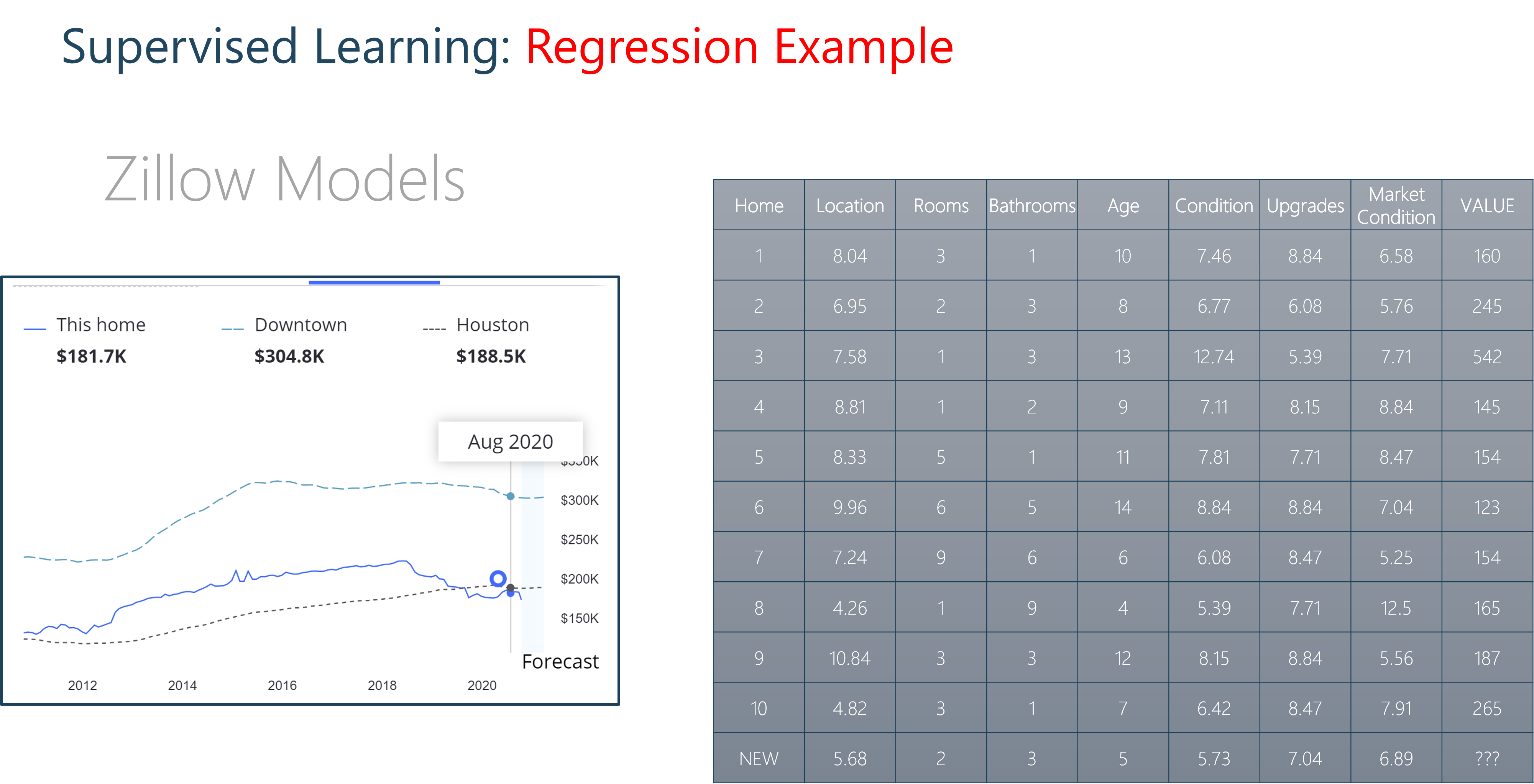
Housing Prices Example

We can imagine this scenario with housing prices. Envision a mixed dataset of continuous and discrete independent variables. Some features could be continuous, floating point values like location ranking and housing condition. Others could be discrete like the number of rooms or bathrooms. We could take these features and use them to predict a house value. This would be a regression model.

1.2 Linear regression fitting with scikit-learn¶

🏋️ Exercise 1: rudimentary EDA¶

What does the data look like? Recall how to visualize data in a pandas dataframe

for every column calculate the:
- skew: df.skew()
- kurtosis: df.kurtosis()
- pearsons correlation with the dependent variable: df.corr()
- number of missing entries df.isnull()
and organize this into a new dataframe

note: pearsons is just one type of correlation, another correlation available to us is spearman which differs from pearsons in that it depends on ranked values rather than their direct quantities, you can read more here

df.isnull().sum()

type                     0
fixed acidity           10
volatile acidity         8
citric acid              3
residual sugar           2
chlorides                2
free sulfur dioxide      0
total sulfur dioxide     0
density                  0
pH                       9
sulphates                4
alcohol                  0
quality                  0
dtype: int64

# Cell for Exercise 1

# part A 
# using df.<method> define the following four variables with the results from
# skew(), kurtosis(), corr() (while selecting for quality), and isnull()
# for isnull() you'll notice the return is a dataframe of booleans. we would
# like to simply know the number of null values for each column. change the
# return of isnull() using the sum() method along the columns

# skew =
# kurt =
# pear =
# null =

# part B
# on line 13, put these results in a list using square brackets and call 
# pd.DataFrame on the list to make your new DataFrame! store it under the
# variable name dff



# part C
# take the transpose of this DataFrame using dff.T. reassign dff to this copy



# part D
# set the column names to 'skew', 'kurtosis', 'pearsons _quality', and 
# 'null count' using dff.columns



# Now return dff to the output to view your hand work
# dff # uncomment this line

I have gone ahead and repeated this exercise with the red vs white wine types:

red = df.loc[df['type'] == 'red']
wht = df.loc[df['type'] == 'white']

def get_summary(df):
  skew = df.skew()
  kurt = df.kurtosis()
  pear = df.corr()['quality']
  null = df.isnull().sum()
  med = df.median()
  men = df.mean()

  dff = pd.DataFrame([skew, kurt, pear, null, med, men])
  dff = dff.T
  dff.columns = ['skew', 'kurtosis', 'pearsons _quality', 'null count', 'median',
                'mean']
  return dff

dffr = get_summary(red)
dffw = get_summary(wht)

desc = pd.concat([dffr, dffw], keys=['red', 'white'])

/tmp/ipykernel_277/2387423026.py:5: FutureWarning: Dropping of nuisance columns in DataFrame reductions (with 'numeric_only=None') is deprecated; in a future version this will raise TypeError.  Select only valid columns before calling the reduction.
  skew = df.skew()
/tmp/ipykernel_277/2387423026.py:6: FutureWarning: Dropping of nuisance columns in DataFrame reductions (with 'numeric_only=None') is deprecated; in a future version this will raise TypeError.  Select only valid columns before calling the reduction.
  kurt = df.kurtosis()
/tmp/ipykernel_277/2387423026.py:9: FutureWarning: Dropping of nuisance columns in DataFrame reductions (with 'numeric_only=None') is deprecated; in a future version this will raise TypeError.  Select only valid columns before calling the reduction.
  med = df.median()
/tmp/ipykernel_277/2387423026.py:10: FutureWarning: Dropping of nuisance columns in DataFrame reductions (with 'numeric_only=None') is deprecated; in a future version this will raise TypeError.  Select only valid columns before calling the reduction.
  men = df.mean()

desc

		skew	kurtosis	pearsons _quality	null count	median	mean
red	fixed acidity	0.982192	1.132624	0.123834	2.0	7.90000	8.322104
	volatile acidity	0.672862	1.226846	-0.390858	1.0	0.52000	0.527738
	citric acid	0.317891	-0.788476	0.226917	1.0	0.26000	0.271145
	residual sugar	4.540655	28.617595	0.013732	0.0	2.20000	2.538806
	chlorides	5.680347	41.715787	-0.128907	0.0	0.07900	0.087467
	free sulfur dioxide	1.250567	2.023562	-0.050656	0.0	14.00000	15.874922
	total sulfur dioxide	1.515531	3.809824	-0.185100	0.0	38.00000	46.467792
	density	0.071288	0.934079	-0.174919	0.0	0.99675	0.996747
	pH	0.194803	0.814690	-0.057094	2.0	3.31000	3.310864
	sulphates	2.429115	11.712632	0.251685	2.0	0.62000	0.658078
	alcohol	0.860829	0.200029	0.476166	0.0	10.20000	10.422983
	quality	0.217802	0.296708	1.000000	0.0	6.00000	5.636023
	type	NaN	NaN	NaN	0.0	NaN	NaN
white	fixed acidity	0.647981	2.176560	-0.114032	8.0	6.80000	6.855532
	volatile acidity	1.578595	5.095526	-0.194976	7.0	0.26000	0.278252
	citric acid	1.284217	6.182036	-0.009194	2.0	0.32000	0.334250
	residual sugar	1.076601	3.469536	-0.097373	2.0	5.20000	6.393250
	chlorides	5.023412	37.560847	-0.210181	2.0	0.04300	0.045778
	free sulfur dioxide	1.406745	11.466342	0.008158	0.0	34.00000	35.308085
	total sulfur dioxide	0.390710	0.571853	-0.174737	0.0	134.00000	138.360657
	density	0.977773	9.793807	-0.307123	0.0	0.99374	0.994027
	pH	0.458402	0.532552	0.098858	7.0	3.18000	3.188203
	sulphates	0.977361	1.589847	0.053690	2.0	0.47000	0.489835
	alcohol	0.487342	-0.698425	0.435575	0.0	10.40000	10.514267
	quality	0.155796	0.216526	1.000000	0.0	6.00000	5.877909
	type	NaN	NaN	NaN	0.0	NaN	NaN

def my_fig(metric=desc.columns):
  fig, ax = plt.subplots(1, 1, figsize=(10,10))
  pd.DataFrame(desc[metric]).unstack()[metric].T.plot(kind='barh', ax=ax)

# interact(my_fig)

🙋 Question 1: Discussion Around EDA Plot¶

What do we think of this plot?

metric = mean, the cholrides values
metric = kurtosis, residual sugar
metric = pearsons _quality, magnitudes and directions
How to improve the plot, what other plots would we like to see?

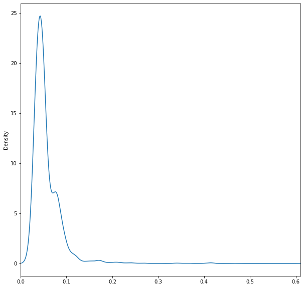
For instance, what if we were really curious about the high kurtosis for chlorides content? What more would we like to glean about the distribution of chloride content?

# we can use df.describe() to take a look at the quantile values and min/max
df['chlorides'].describe()

count    6495.000000
mean        0.056042
std         0.035036
min         0.009000
25%         0.038000
50%         0.047000
75%         0.065000
max         0.611000
Name: chlorides, dtype: float64

# and see how these values appear in a KDE
fig, ax = plt.subplots(1,1,figsize=(10,10))
df['chlorides'].plot(kind='kde',ax=ax)
ax.set_xlim(0,.61)

(0.0, 0.61)

png

# lastly we may want to look at the raw values themselves. We can sort them 
# too view outliers
df['chlorides'].sort_values(ascending=False)[:50]

5156    0.611
5049    0.610
5004    0.467
4979    0.464
5590    0.422
6268    0.415
6270    0.415
5652    0.415
6217    0.414
5949    0.414
5349    0.413
6158    0.403
4981    0.401
5628    0.387
6063    0.369
4915    0.368
5067    0.360
5179    0.358
484     0.346
5189    0.343
4917    0.341
5124    0.337
4940    0.332
1217    0.301
687     0.290
4473    0.271
5079    0.270
6272    0.267
5138    0.263
1865    0.255
5466    0.250
1034    0.244
5674    0.243
5675    0.241
683     0.240
1638    0.239
5045    0.236
6456    0.235
6468    0.230
5465    0.226
5464    0.226
5564    0.222
2186    0.217
5996    0.216
6333    0.214
5206    0.214
6332    0.214
5205    0.213
4497    0.212
1835    0.211
Name: chlorides, dtype: float64

1.2.2 Visualizing the data set - motivating regression analysis¶

In order to demonstrate simple linear regression with this dataset we will look at two particular features: fixed acidity and density.

We can create a scatter plot of fixed acidity vs density for the red wine in the dataset using df.plot() and see that there appears to be a general trend between the two features:

fig, ax = plt.subplots(1, 1, figsize=(5,5))
df.loc[df['type'] == 'red'].plot(x='fixed acidity', y='density', ax=ax, 
                                 ls='', marker='.')

<AxesSubplot:xlabel='fixed acidity'>

png

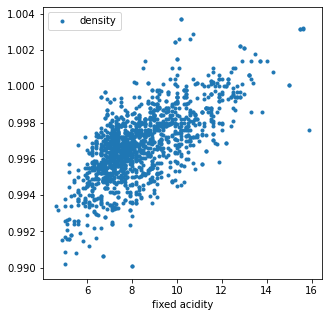
Now the question is: How do we quantify this trend?

1.2.3 Estimating the regression coefficients¶

It looks like density increases with fixed acidity following a line, maybe something like

$y(x)= m \cdot x + b \;\;\;\;\;\;\;\; \sf{eq. 1}$

with $ y=\sf density $, $x=\sf fixed \space acidity$, and $m$ the slope and $b$ the intercept.

To solve the problem, we need to find the values of $b$ and $m$ in equation 1 to best fit the data. This is called linear regression.

In linear regression our goal is to minimize the error between computed values of positions $y^{\sf calc}(x_i)\equiv y^{\sf calc}_i$ and known values $y^{\sf exact}(x_i)\equiv y^{\sf exact}_i$.

In Ordinary Least Squares the error term we try to minimize is called the residual sum of squares. We find $b$ and $m$ which lead to lowest value of

$\epsilon (m,b) =SS_{\sf res}=\sum_{i=1}^{N}\left(y^{\sf exact}_i - y^{\sf calc}_i\right)^2 = \sum_{i=1}^{N}\left(y^{\sf exact}_i - m\cdot x_i - b \right)^2\;\;\;\;\;\;\;\;\;\;\;\sf{eq. 2}$

To find out more see e.g. https://en.wikipedia.org/wiki/Simple_linear_regression

Using some calculus, we can solve for $b$ and $m$ analytically:

$m = \frac{\sum_{i=1}^n{(x_i - \bar{x})(y_i - \bar{y})}}{\sum_{i=1}^n{(x_i - \bar{x})^2}}$

$b = \bar{y} - m\bar{x}$

Note that for multivariate regression, the coefficients can be solved analytically as well 😎

🙋 Question 2: linear regression loss function¶

Do we always want m and b to be large positive numbers so as to minimize eq. 2?

Luckily scikit-learn contains many functions related to regression including linear regression.

The function we will use is called LinearRegression() .

# Create linear regression object
model = linear_model.LinearRegression()

# Use model to fit to the data, the x values are densities and the y values are fixed acidity
# Note that we need to reshape the vectors to be of the shape x - (n_samples, n_features) and y (n_samples, n_targets)
x = red['density'].values.reshape(-1, 1)
y = red['fixed acidity'].values.reshape(-1, 1)

print(red['density'].values.shape, red['fixed acidity'].values.shape)
print(x.shape, y.shape)

(1599,) (1599,)
(1599, 1) (1599, 1)

What happens when we try to fit the data as is?

# Fit to the data
# model.fit(x, y)

🏋️ Exercise 2: drop Null Values (and practice pandas operations)¶

Let's look back at our dataset description dataframe above, what do we notice, what contains null values?

There are several strategies for dealing with null values. For now let's take the simplest case, and drop rows in our dataframe that contain null

# Cell for Exercise 2
# For this templated exercise you are going to complete everything in one line 
# of code, but we are going to break it up into steps. So for each part (A, B,
# etc.) paste your answer from the previous part to begin (your opertaions will
# read from left to right)

# step A
# select the 'density' and 'fixed acidity' columns of red. make sure the return
# is a dataframe

# step B
# now use the dropna() method on axis 0 (the rows) to drop any null values 

# step B
# select column 'density'

# step C
# select the values

# step D
# reshape the result with an empty second dimension using .reshape() and store
# the result under variable x

# repeat the same process with 'fixed acidity' and variable y

Now that we have our x and y arrays we can fit using ScikitLearn

x = red[['density', 'fixed acidity']].dropna(axis=0)['density'].values.reshape(-1,1)
y = red[['density', 'fixed acidity']].dropna(axis=0)['fixed acidity'].values.reshape(-1,1)

🙋 Question 3: why do we drop null values across both columns?¶

Notice in the above cell how we selected both density and fixed acidity before calling dropna? Why did we do that? Why didn't we just select density in the x variable case and fixed acidity in the y variable case?

# Fit to the data
model.fit(x, y)

# Extract the values of interest
m = model.coef_[0][0]
b = model.intercept_[0]

# Print the slope m and intercept b
print('Scikit learn - Slope: ', m , 'Intercept: ', b )

Scikit learn - Slope:  616.01314280661 Intercept:  -605.6880086750523

🏋️ Exercise 3: calculating y_pred¶

Estimate the values of $y$ by using your fitted parameters. Hint: Use your model.coef_ and model.intercept_ parameters to estimate y_pred following equation 1

# define y_pred in terms of m, x, and b
# y_pred = 

# uncomment the following lines!
# fig, ax = plt.subplots(1,1, figsize=(10,10))
# ax.plot(x, y_pred, ls='', marker='*')
# ax.plot(x, y, ls='', marker='.')

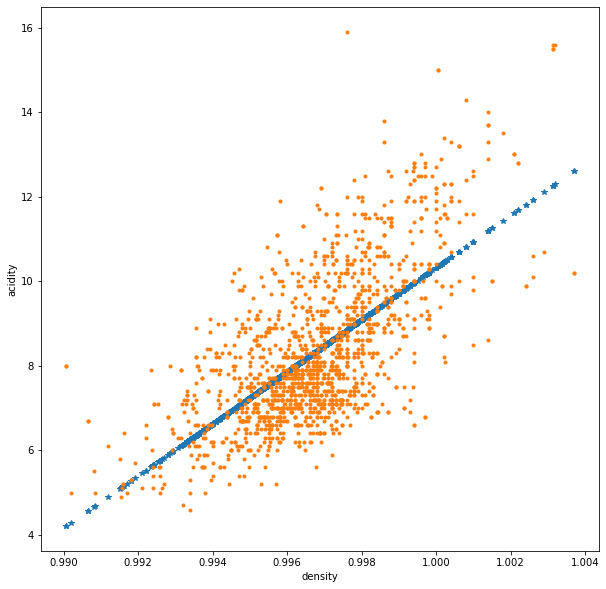
We can also return predictions directly with the model object using the predict() method

note: it is great to get in the habit of utilizing model outputs this way, as the API will be similar across all scikit-learn models (and sometimes models in other libraries as well!)

# Another way to get this is using the model.predict function
y_pred = model.predict(x)
fig, ax = plt.subplots(1,1, figsize=(10,10))
ax.plot(x, y_pred, ls='', marker='*')
ax.plot(x, y, ls='', marker='.')
ax.set_ylabel('acidity')
ax.set_xlabel('density')

Text(0.5, 0, 'density')

png

1.3 Error and topics of model fitting (assessing model accuracy)¶

1.3.1 Measuring the quality of fit¶

1.3.1.1 Mean Squared Error¶

The plot in Section 1.2.3 looks good, but numerically what is our error? What is the mean value of $\epsilon$, i.e. the Mean Squared Error (MSE)?

${\sf MSE}=\epsilon_{\sf ave} = \frac{\sum_{i=1}^{N_{\sf times}}\left(y^{\sf exact}_i - m\cdot t_i - b \right)^2}{N_{\sf times}}\;\;\;\;\;\sf eq. 3$

# The mean squared error
print('Mean squared error: %.2f' % mean_squared_error(y, y_pred))

Mean squared error: 1.68

1.3.1.2 R-square¶

Another way to measure error is the regression score, $R^2$. $R^2$ is generally defined as the ratio of the total sum of squares $SS_{\sf tot}$ to the residual sum of squares $SS_{\sf res}$:

$SS_{\sf tot}=\sum_{i=1}^{N} \left(y^{\sf exact}_i-\bar{y}\right)^2\;\;\;\;\; \sf eq. 4$ $SS_{\sf res}=\sum_{i=1}^{N} \left(y^{\sf exact}_i - y^{\sf calc}_i\right)^2\;\;\;\;\; \sf eq. 5$ $R^2 = 1 - {SS_{\sf res}\over SS_{\sf tot}} \;\;\;\;\;\; \sf eq. 6$

In eq. 4, $\bar{y}=\sum_i y^{\sf exact}_i/N$ is the average value of y for $N$ points. The best value of $R^2$ is 1 but it can also take a negative value if the error is large.

See all the different regression metrics here.

🙋 Question 4: lets understand $R^2$¶

Do we need a large value of $SS_{\sf tot}$ to minimize $R^2$ - is this something which we have the power to control?

# Print the coefficient of determination - 1 is perfect prediction
print('Coefficient of determination: %.2f' % r2_score(y, y_pred))

Coefficient of determination: 0.45

🍒 1.3.1.3 Enrichment: Residual Standard Error¶

the residual standard error (RSE) is an estimate of the standard deviation of the irreducible error (described more in Model Selection and Validation)

$RSE = \sqrt{\frac{1}{n-2}RSS}$

In effect, the RSE tells us that even if we were to find the true values of $b$ and $m$ in our linear model, this is by how much our estimates of $y$ based on $x$ would be off.

🍒 1.3.2 Enrichment: Assessing the accuracy of the coefficient estimates¶

1.3.2.1 Standard errors¶

The difference between our sample and the population data is often a question in statistical learning (covered more in session Model Selection and Validation). As an estimate on how deviant our sample mean may be from the true population mean, we can calculate he standard error of the sample mean:

$SE(\hat{\mu})^2 = \frac{\sigma^2}{N}$

where $\sigma$ is the standard deviation of each of the realizations of $y_i$ with $Y$.

We can similarly calculate standard errors for our estimation coefficients:

$SE(\hat{b})^2 = \sigma^2 [\frac{1}{n} + \frac{\bar{x}^2}{\sum_{i=1}^n{(x_i - \bar{x})^2}}]$

$SE(\hat{m})^2 = \frac{\sigma^2}{\sum_{i=1}^n{(x_i - \bar{x})^2}}$

In practice, $\sigma$ is estimated as the residual standard error:

$RSE = \sqrt{RSS/(n-2)}$

We might observe:

$SE(\hat{b})^2$ would equal $SE(\hat{\mu})^2$ if $\bar{x}$ were 0 (and $\hat{b}$ would equal $\bar{y}$)
and the error associated with $m$ and $b$ would be smaller with the more spread we have in $x_i$ (intuitively a spread in $x_i$ gives us more leverage)

1.3.2.2 Confidence intervals¶

These standard errors can be used to compute confidence intervals. A 95% confidence interval is defined as a range a values that with a 95% probability contain the true value of the predicted parameter.

$\hat{b} \space ± \space 2 SE(\hat{b})$

and

$\hat{m} \space ± \space 2 SE(\hat{m})$

# b_hat
print(f"b: {b:.2e}")
print(f"m: {m:.2e}", end="\n\n")
n = y.shape[0]
print(f"n: {n}")
x_bar = np.mean(x)
print(f"x_bar: {x_bar:.2e}")
RSE = np.sqrt(r2_score(y, y_pred)/(n-2))
print(f"RSE: {RSE:.2e}", end="\n\n")

SE_b = np.sqrt(RSE**2 * ((1/n) + x_bar**2/np.sum((x-x_bar)**2)))
print(f"SE_b: {SE_b:.2e}")

SE_m = np.sqrt(RSE**2/np.sum((x-x_bar)**2))
print(f"SE_m: {SE_m:.2e}")

b: -6.06e+02
m: 6.16e+02

n: 1597
x_bar: 9.97e-01
RSE: 1.67e-02

SE_b: 2.21e-01
SE_m: 2.22e-01

The confidence interval around the regression line takes on a similar form

$SE(\hat{y})^2 = (\frac{\sum_{i=1}^n{(y_i - \hat{y})^2}} {n-2}) (\frac{1}{n} + \frac{(x-\bar{x})^2} {\sum_{i=1}^n{(x_i - \bar{x})^2}})$

and then $\hat{y}$ can be described as

$\hat{y}_h ± t_{\alpha/2,n-2} SE(\hat{y})$

where $t$ is the calculated critical t-value at the corresponding confidence interval and degrees of freedom (we can obtain this from scipy)

def calc_SE_y(x, y, m, b):
    y_hat = m*x+b
    x_bar = np.mean(x)
    n = x.shape[0]

    return np.sqrt((np.sum((y-y_hat)**2))/(n-2)) \
            * np.sqrt((1/n) + ((x-x_bar)**2 / (np.sum((x-x_bar)**2))))

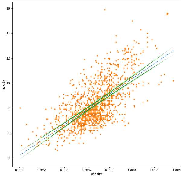
x_line = np.linspace(min(x), max(x), 100)
y_line = m*x_line+b
fig, ax = plt.subplots(1,1, figsize=(10,10))
ax.plot(x_line, y_line, ls='--')
ax.plot(x, y, ls='', marker='.')

SE_y = calc_SE_y(x, y, m, b)
y_line = m*x+b
ct = scipy.stats.t.ppf(q=(0.975), df=(n-2))

### upper CI
y_up = y_line + ct * SE_y
ax.plot(x, y_up, ls='-.', marker='', color='tab:green', lw=.1)

### lower CI
y_down = y_line - ct * SE_y
ax.plot(x, y_down, ls='-.', marker='', color='tab:green', lw=.1)

ax.set_ylabel('acidity')
ax.set_xlabel('density')

Text(0.5, 0, 'density')

png

1.3.2.3 Hypothesis testing¶

standard errors can also be used to perform hypothesis tests on the coefficients. The most common hypothesis test involves testing the null hypothesis of

$H_0:$ There is no relationship between X and Y

versus the alternative hypothesis

$H_\alpha:$ There is some relationship between X and Y

This is equivalent to

$H_0: m = 0$

and

$H_\alpha: m ≠ 0$

since if $m = 0$ there is no relationship between X and Y. We need to assess if our $m$ is sufficiently far from 0. Intuitively, this would also require us to consider the error $SE(\hat{m})$. In practice we compute a t-statistic

$t = \frac{\hat{m}-0}{SE(\hat{m})}$

which measures the number of standard deviations $m$ is from 0. Associated with this statistic, we determine a p-value (a "probability"-value) that tells us the probability of observing any value equal to $|t|$ or larger, assuming the null hypothesis of $m=0$. Hence, if we determine a small p-value, we can conclude that it is unlikely that there is no relationship between X and Y.

t = m/SE_m
print(t)

2777.3933859895524

scipy.stats.t.sf(x=t, df=n-2)

0.0

We see that with this data it is very unlikely that there is no relationship between X and Y!

1.3.3 Corollaries with classification models¶

For classification tasks, we typically assess accuracy vs MSE or R-square, since we are dealing with categorical rather than numerical predictions.

What is accuracy? It is defined as the ratio of True assignments to all assignments. For a binary positive/negative classification task this can be written as the following:

$Acc = \frac{T_p + T_n}{F_p + F_n + T_p + T_n}$

Where $T$ is True, $F$ is false, $p$ is positive, $n$ is negative

Just as a quick example, we can perform this type of task on our wine dataset by predicting on quality, which is a discrete 3-9 quality score:

y_train = df['type'].values.reshape(-1,1)
x_train = df['quality'].values.reshape(-1,1)

# train a logistic regression model on the training set
from sklearn.linear_model import LogisticRegression

# instantiate model
logreg = LogisticRegression()

# fit model
logreg.fit(x_train, y_train)

/home/wbeckner/anaconda3/envs/py39/lib/python3.9/site-packages/sklearn/utils/validation.py:993: DataConversionWarning: A column-vector y was passed when a 1d array was expected. Please change the shape of y to (n_samples, ), for example using ravel().
  y = column_or_1d(y, warn=True)





LogisticRegression()

# make class predictions for the testing set
y_pred_class = logreg.predict(x_train)

# calculate accuracy
from sklearn import metrics
print(metrics.accuracy_score(y_train, y_pred_class))

0.7538864091118977

🙋 Question 5: What is variance vs total sum of squares vs standard deviation?¶

1.3.4 Beyond a single input feature¶

(also: quick appreciative beat for folding in domain area expertise into our models and features)

The acidity of the wine (the dependent variable v) could depend on:

potassium from the soil (increases alkalinity)
unripe grapes (increases acidity)
grapes grown in colder climates or reduced sunshine create less sugar (increases acidity)
preprocessing such as adding tartaric acid to the grape juice before fermentation (increases acidity)
malolactic fermentation (reduces acidity)
+ others

So in our lab today we will look at folding in additional variables in our dataset into the model

1.4 Multivariate regression¶

Let's now turn our attention to wine quality.

The value we aim to predict or evaluate is the quality of each wine in our dataset. This is our dependent variable. We will look at how this is related to the 12 other independent variables, also known as input features. We're going to do this with only the red wine data

red.head()

	type	fixed acidity	volatile acidity	citric acid	residual sugar	chlorides	free sulfur dioxide	total sulfur dioxide	density	pH	sulphates	alcohol	quality
4898	red	7.4	0.70	0.00	1.9	0.076	11.0	34.0	0.9978	3.51	0.56	9.4	5
4899	red	7.8	0.88	0.00	2.6	0.098	25.0	67.0	0.9968	3.20	0.68	9.8	5
4900	red	7.8	0.76	0.04	2.3	0.092	15.0	54.0	0.9970	3.26	0.65	9.8	5
4901	red	11.2	0.28	0.56	1.9	0.075	17.0	60.0	0.9980	3.16	0.58	9.8	6
4902	red	7.4	0.70	0.00	1.9	0.076	11.0	34.0	0.9978	3.51	0.56	9.4	5

1.4.1 Linear regression with all input fields¶

For this example, notice we have a categorical data variable in the 'type' column. We will ignore this for now, and only work with our red wines. In the future we will discuss how to deal with categorical variable such as this in a mathematical representation.

# this is a list of all our features or independent variables
features = list(red.columns[1:])

# we're going to remove our target or dependent variable, density from this
# list
features.remove('density')

# now we define X and y according to these lists of names
X = red.dropna(axis=0)[features].values
y = red.dropna(axis=0)['density'].values

# we will talk about scaling/centering our data at a later time
X = (X - X.mean(axis=0)) / X.std(axis=0)

red.isnull().sum(axis=0) # we are getting rid of some nasty nulls!

type                    0
fixed acidity           2
volatile acidity        1
citric acid             1
residual sugar          0
chlorides               0
free sulfur dioxide     0
total sulfur dioxide    0
density                 0
pH                      2
sulphates               2
alcohol                 0
quality                 0
dtype: int64

# Create linear regression object - note that we are using all the input features
model = linear_model.LinearRegression()
model.fit(X, y)
y_hat = model.predict(X)

Let's see what the coefficients look like ...

print("Fit coefficients: \n", model.coef_, "\nNumber of coefficients:", len(model.coef_))

Fit coefficients: 
 [ 1.64059336e-03  1.23999138e-04  1.16115898e-05  5.83002013e-04
  8.35961822e-05 -9.17472420e-05  8.61246026e-05  7.80966358e-04
  2.24558885e-04 -9.80600257e-04 -1.75587885e-05] 
Number of coefficients: 11

We have 11 !!! That's because we are regressing respect to all 11 independent variables!!!

So now, $y_{\sf calc}= m_1x_1 +\, m_2x_2 \,+ \,m_3x_3 \,+\,... \,+ \,b =\sum_{i=1}^{13}m_i x_i + b\;\;\;\;\; \sf eq. 7$

print("We have 11 slopes / weights:\n\n", model.coef_)
print("\nAnd one intercept: ", model.intercept_)

We have 11 slopes / weights:

 [ 1.64059336e-03  1.23999138e-04  1.16115898e-05  5.83002013e-04
  8.35961822e-05 -9.17472420e-05  8.61246026e-05  7.80966358e-04
  2.24558885e-04 -9.80600257e-04 -1.75587885e-05]

And one intercept:  0.9967517451349656

# This size should match the number of columns in X
if len(X[0]) == len(model.coef_):
    print("All good! The number of coefficients matches the number of input features.")
else:
    print("Hmm .. something strange is going on.")

All good! The number of coefficients matches the number of input features.

🏋️ Exercise 4: evaluate the error¶

Let's evaluate the error by computing the MSE and $R^2$ metrics (see eq. 3 and 6).

# The mean squared error

# part A 
# calculate the MSE using mean_squared_error()
# mse = 

# part B
# calculate the R square using r2_score()
# r2 = 

# print('Mean squared error: {:.2f}'.format(mse))
# print('Coefficient of determination: {:.2f}'.format(r2))

🏋️ Exercise 5: make a plot of y actual vs y predicted¶

We can also look at how well the computed values match the true values graphically by generating a scatterplot.

# generate a plot of y predicted vs y actual using plt.plot()
# remember you must set ls to an empty string and marker to some marker style

# plt.plot()
plt.title("Linear regression - computed values on entire data set", fontsize=16)
plt.xlabel("y$^{\sf calc}$")
plt.ylabel("y$^{\sf true}$")
plt.show()

png

🍒 1.4.2 Enrichment: Splitting into train and test sets¶

note: more of this topic is covered in Model Selection and Validation

To see whether we can predict, we will carry out our regression only on a part, 80%, of the full data set. This part is called the training data. We will then test the trained model to predict the rest of the data, 20% - the test data. The function which fits won't see the test data until it has to predict it.

We start by splitting out data using scikit-learn's train_test_split() function:

X_train, X_test, y_train, y_test = train_test_split(X, y, 
                                                    test_size=0.20,
                                                    random_state=42)

Now we check the size of y_train and y_test , the sum should be the size of y! If this works then we move on and carry out regression but we only use the training data!

if len(y_test)+len(y_train) == len(y):

    print('All good, ready to to go and regress!\n')

    # Carry out linear regression
    print('Running linear regression algorithm on the training set\n')
    model = linear_model.LinearRegression()
    model.fit(X_train, y_train)
    print('Fit coefficients and intercept:\n\n', model.coef_, '\n\n', model.intercept_ )

    # Predict on the test set
    y_pred_test = model.predict(X_test)

All good, ready to to go and regress!

Running linear regression algorithm on the training set

Fit coefficients and intercept:

 [ 1.62385613e-03  1.10578142e-04  7.75216492e-07  5.87755741e-04
  7.65190323e-05 -1.03490059e-04  8.87357873e-05  7.79083342e-04
  2.23534769e-04 -9.99858829e-04  5.85256438e-06]

 0.9967531628434799

Now we can plot our predicted values to see how accurate we are in predicting. We will generate a scatterplot and computing the MSE and $R^2$ metrics of error.

sns.scatterplot(x=y_pred_test, y=y_test, color="mediumvioletred", s=50)

plt.title("Linear regression - predict test set", fontsize=16)
plt.xlabel("y$^{\sf calc}$")
plt.ylabel("y$^{\sf true}$")
plt.show()

print('Mean squared error: %.2e' % mean_squared_error(y_test, y_pred_test))
print('Coefficient of determination: %.2f' % r2_score(y_test, y_pred_test))

png

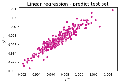
Mean squared error: 5.45e-07
Coefficient of determination: 0.87

🍒 1.4.3 Enrichment: Some important questions¶

is at least one of the predictors useful in estimating y?
- We'll see related topics in Inferential Statistics
Do we need all the predictors or only some of them?
- We'll see related topics in Feature Engineering
How do we assess goodness of fit?
How accurate is any given prediction?

1.4.3.1 Is there a relationship between X and y?¶

This question is similar to the hypothesis test we had as an enrichment topic in simple linear regression. To be formulaic:

$H_0 : \beta_1 = \beta_2 = ... = \beta_p = 0$

$H_\alpha : at \space least \space one \space \beta_j \space is \space non-zero$

To answer this question we perform an F-statistic

$F = \frac{(TSS - RSS)/p}{RSS/(n-p-1)}$

where $p$ is the number of predictors. With this F-statistic, we are expecting that if there is no relationship between the predictors and target variable the ratio would converge to 1, since both numerator and denominator would evaluate to simply the variance of the data. On the other hand, if there is a relationship the numerator (the variance captured by the model over the number of predictors) should evaluate to something greater than the variance of the data.

Now you might ask, why can't single out every predictor and perform the hypothesis testing we saw before?! Well, by sheer chance, we may incorrectly throw out the null hypothesis. Take an extreme example, if we have 100 predictors, with a confidence level of 0.05 we would by chance alone accept 5 of those 100 predictors, even if they have no relationship to Y. This is where the F-statistic comes in handy (it is worth noting however, that even the F-statistic can't handle $p$ > $n$ for which there is no solution!)

y_bar = np.mean(y)
y_hat = model.predict(X)
RSS = np.sum((y-y_hat)**2)
TSS = np.sum((y-y_bar)**2)
p = X.shape[1]
n = X.shape[0]
F = (TSS-RSS)/p / (RSS/(n-p-1))
print(f"{F:.2f}")

767.86

# http://pytolearn.csd.auth.gr/d1-hyptest/11/f-distro.html
# dfn = degrees of freedom in the numerator
# dfd = degrees of freedom in the denominator
scipy.stats.f.sf(x=t, dfn=p, dfd=(n-p-1))

0.0

with this result we can be fairly certain 1 or more of the prdictors is related to the target variable!

1.4.2.2 What are the important variables?¶

the process of determining which of the variables are associated with y is known as variable selection. One approach, is to iteratively select every combination of variables, perform the regression, and use some metric of goodness of fit to determine which subset of p is the best. However this is $2^p$ combinations to try, which quickly blows up. Instead we typically perform one of three approaches

Forward selection
- start with an intercept model. Add a single variable, keep the one that results in the lowest RSS. Repeat. Can always be used no matter how large p is. This is also a greedy approach.
Backward selection
- start with all predictors in the model. Remove the predictor with the largest p-value. Stop when all p-values are below some threshold. Can't be used if p > n.
Mixed selection
- a combination of 1 and 2. start with an intercept model. continue as in 1 accept now, if any predictor p-value rises above some threshold, remove that predictor. This approach counteracts some of the greediness of approach 1.

1.4.2.3 How do we assess goodness of fit?¶

Two of the most common measures of goodness of fit are $RSE$ and $R^2$. As it turns out, however, $R^2$ will always increase with more predictors. The $RSE$ defined for multivariate models accounts for the additional p:

$RSE = \sqrt{\frac{1}{n-p-1} RSS}$

and thus can be used in tandem with $R^2$ to assess whether the additional parameter is worth it or not.

Lastly, it is worth noting that visual approaches can lend a hand where simple test values can not (think Anscombe's quartet).

1.4.2.4 How accurate is any given prediction?¶

We used confidence intervals to quantify the uncertainty in the estimate for $f(X)$. To assess the uncertainty around a particular prediction we use prediction intervals. A prediction interval will always be wider than a confidence interval because it incorporates both the uncertainty in the regression estimate (reducible error or sampling error) and uncertainty in how much an individual point will deviate from the solution surface (the irreducible error).

Put another way, with the confidence interval we expect the average response of y to fall within the calculated interval 95% of the time, however we sample the population data. Whereas we expect an individual response, y, to fall within the calculated prediction interval 95% of the time, however we sample the population data.

1.5 Major assumptions of linear regression¶

There are two major assumptions of linear regression: that the predictors are additive, and that the relationships between X and y are linear.

We can combat these assumptions, however, through feature engineering, a topic we discuss later on but briefly we will mention here. In the additive case, predictors that are suspected to have some interaction affect can be combined to produce a new feature, i.e. $X_{new} = X_2*X_2$. On the linearity case, we can again engineer a new feature, i.e. $X_{new} = X_1^2$.

🍒 1.6 Enrichment: Potential problems with linear regression¶

Non-linearity of the response-predictor relationships.
- plot the residuals (observe there is no pattern)
Correlation of error terms.
- standard errors are predicated on no correlation of error terms. Extreme example: we double our data, n is now twice as large, and our confidence intervals narrower by a factor of $\sqrt(2)$!
- a frequent problem in time series data
  - plot residuals as a function of time (observe there is no pattern)
Non-constant variance of error terms (heteroscedasticity).
- standard errors, hypothesis tests, and confidence intervals rely on this assumption
- a funnel shape in the residuals indicates heteroscedasticity
- can transform, $\log{y}$
Outliers.
- unusual values in response variable
- check residual plot
- potentially remove datapoint
High-leverage points.
- unusual values in predictor variable
- will bias the least squares line
- problem can be hard to observe in multilinear regression (when a combination of predictors accounts for the leverage)
Collinearity.
- refers to when two or more variables are closely related to one another
- reduces the accuracy of esimates for coefficients
- increases standard error of estimates for coefficients. it then reduces the t-statistic and may result in type-2 error, false negative. This means it reduces the power of the hypothesis test, the probability of correctly detecting a non-zero coefficient.
- look at the correlation matrix of variables
- for multicolinearity compute the variance inflation factor (VIF)
  - $1/(1-R^2)$ where the regression is performed against the indicated predictor across all other predictors
- remove features with a VIF above 5-10

We will discuss many of these in the session on Feature Engineering

🍒 1.7 Enrichment: Other regression algorithms¶

There are many other regression algorithms the two we want to highlight here are Ridge, LASSO, and Elastic Net. They differ by an added term to the loss function. Let's review. Eq. 2 expanded to multivariate form yields:

$\sum_{i=1}^{N}(y_i - \sum_{j=1}^{P}x_{ij}\beta_{j})^2$

for Ridge regression, we add a regularization term known as L2 regularization:

$\sum_{i=1}^{N}(y_i - \sum_{j=1}^{P}x_{ij}\beta_{j})^2 + \lambda \sum_{j=1}^{P}\beta_{j}^2$

for LASSO (Least Absolute Shrinkage and Selection Operator) we add L1 regularization:

$\sum_{i=1}^{N}(y_i - \sum_{j=1}^{P}x_{ij}\beta_{j})^2 + \lambda \sum_{j=1}^{P}|\beta_{j}|$

The key difference here is that LASSO will allow coefficients to shrink to 0 while Ridge regression will not. Elastic Net is a combination of these two regularization methods.

model = linear_model.Ridge()
model.fit(X_train, y_train)
print('Fit coefficients and intercept:\n\n', model.coef_, '\n\n', model.intercept_ )

# Predict on the test set
y_hat_test = model.predict(X_test)

Fit coefficients and intercept:

 [ 1.61930554e-03  1.11227142e-04  2.64709094e-06  5.87271456e-04
  7.58510569e-05 -1.02851782e-04  8.76686650e-05  7.75641517e-04
  2.23315063e-04 -9.98653815e-04  5.26839010e-06]

 0.9967531358810221

sns.scatterplot(x=y_hat_test, y=y_test, color="lightseagreen", s=50)
plt.title("Ridge regression - predict test set",fontsize=16)
plt.xlabel("y$^{\sf calc}$")
plt.ylabel("y$^{\sf true}$")
plt.show()

print('Mean squared error: %.2f' % mean_squared_error(y_test, y_hat_test))
print('Coefficient of determination: %.2f' % r2_score(y_test, y_hat_test))

png

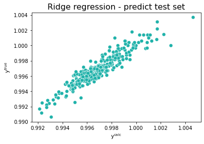
Mean squared error: 0.00
Coefficient of determination: 0.87

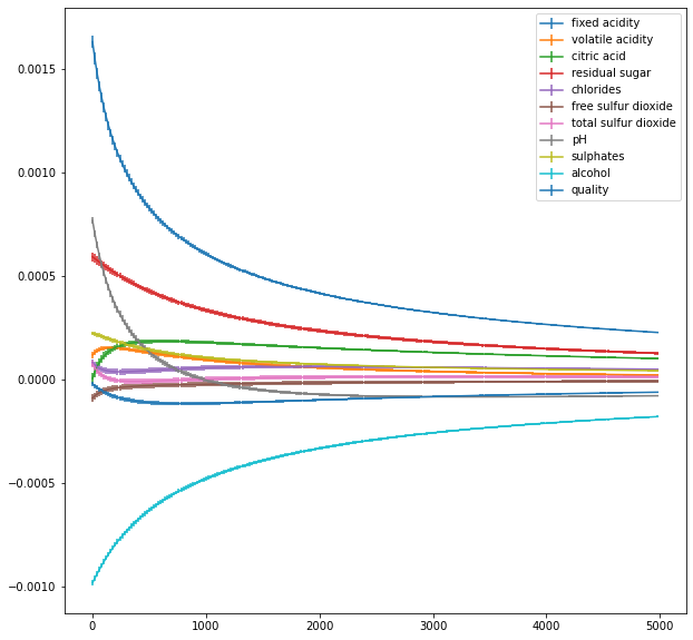
🏋️ Exercise 6: Tune Hyperparameter for Ridge Regression¶

Use the docstring to peak into the hyperparameters for Ridge Regression. What is the optimal value of lambda?

Plot the $\beta$ values vs $\lambda$ from the results of your analysis

# cell for exercise 3
out_lambdas = []
out_coefs = []
out_scores = []
for i in range(10):
  lambdas = []
  coefs = []
  scores = []
  X_train, X_test, y_train, y_test = train_test_split(X, y, 
                                                    test_size=0.20)
  for lamb in range(1,int(5e3),20):
    model = linear_model.Ridge(alpha=lamb)
    model.fit(X_train, y_train)
    lambdas.append(lamb)
    coefs.append(model.coef_)
    scores.append(r2_score(y_test, model.predict(X_test)))
    # print('MSE: %.4f' % mean_squared_error(y_test, model.predict(X_test)))
    # print('R2: %.4f' % r2_score(y_test, model.predict(X_test)))
  out_lambdas.append(lambdas)
  out_coefs.append(coefs)
  out_scores.append(scores)

coef_means = np.array(out_coefs).mean(axis=0)
coef_stds = np.array(out_coefs).std(axis=0)
results_means = pd.DataFrame(coef_means,columns=features)
results_stds = pd.DataFrame(coef_stds,columns=features)
results_means['lambda'] = [i for i in lambdas]

fig, ax = plt.subplots(1,1,figsize=(10,10))
for feat in features:
  ax.errorbar([i for i in lambdas], results_means[feat], yerr=results_stds[feat], label=feat)
# results.plot('lambda', 'scores', ax=ax[1])
ax.legend()

<matplotlib.legend.Legend at 0x7fdd72270fd0>

png

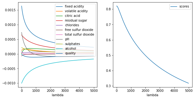
results = pd.DataFrame(coefs,columns=features)
results['lambda'] = [i for i in lambdas]
results['scores'] = scores

fig, ax = plt.subplots(1,2,figsize=(10,5))
for feat in features:
  results.plot('lambda', feat, ax=ax[0])
results.plot('lambda', 'scores', ax=ax[1])

<AxesSubplot:xlabel='lambda'>

png

🍒 1.8 Enrichment: Additional Regression Exercises¶

Problem 1) Number and choice of input features¶

Load the red wine dataset and evaluate how the linear regression predictions changes as you change the number and choice of input features. The total number of columns in X is 11 and each column represents a specific input feature.
Estimate the MSE

print(X_train.shape)

(1274, 11)

If you want to use the first 5 features you could proceed as following:

X_train_five = X_train[:,0:5]
X_test_five = X_test[:,0:5]

Check that the new variables have the shape your expect

print(X_train_five.shape)
print(X_test_five.shape)

(1274, 5)
(319, 5)

Now you can use these to train your linear regression model and repeat for different numbers or sets of input features! Note that you do not need to change the output feature! It's size is independent from the number of input features, yet recall that its length is the same as the number of values per input feature.

Questions to think about while you work on this problem - How many input feature variables does one need? Is there a maximum or minimum number? - Could one input feature variable be better than the rest? - What if values are missing for one of the input feature variables - is it still worth using it? - Can you use L1 or L2 to determine these optimum features more quickly?

Problem 2) Type of regression algorithm¶

Try using other types of linear regression methods on the wine dataset: the LASSO model and the Elastic net model which are described by the

sklearn.linear_model.ElasticNet()
sklearn.linear_model.Lasso()

scikit-learn functions.

For more detail see ElasticNet and Lasso.

Questions to think about while you work on this problem - How does the error change with each model? - Which model seems to perform best? - How can you optimize the hyperparameter, $\lambda$ - Does one model do better than the other at determining which input features are more important? - How about non linear regression / what if the data does not follow a line? - How do the bias and variance change for each model

from sklearn.linear_model import ElasticNet
from sklearn.linear_model import Lasso
from sklearn.linear_model import Ridge
from sklearn.linear_model import LinearRegression

for model in [ElasticNet, Lasso, Ridge, LinearRegression]:
  model = model()
  model.fit(X_train, y_train)
  print(str(model))
  print('Mean squared error: %.ef' % mean_squared_error(y_test, model.predict(X_test)))
  print('Coefficient of determination: %.2f' % r2_score(y_test, model.predict(X_test)))
  print()

ElasticNet()
Mean squared error: 4e-06f
Coefficient of determination: -0.00

Lasso()
Mean squared error: 4e-06f
Coefficient of determination: -0.00

Ridge()
Mean squared error: 7e-07f
Coefficient of determination: 0.83

LinearRegression()
Mean squared error: 7e-07f
Coefficient of determination: 0.83

References¶

Linear Regression To find out more see simple linear regression
scikit-learn
Pearson correlation To find out more see pearson
Irreducible error, bias and variance
- Great Coursera videos here and here

Data Science Foundations Session 1: Regression and Analysis¶

1.0 Preparing Environment and Importing Data¶

1.0.1 Import Packages¶

1.0.2 Load Dataset¶

1.1 What is regression?¶

1.2 Linear regression fitting with scikit-learn¶

🏋️ Exercise 1: rudimentary EDA¶

🙋 Question 1: Discussion Around EDA Plot¶

1.2.2 Visualizing the data set - motivating regression analysis¶

1.2.3 Estimating the regression coefficients¶

🙋 Question 2: linear regression loss function¶

🏋️ Exercise 2: drop Null Values (and practice pandas operations)¶

🙋 Question 3: why do we drop null values across both columns?¶

🏋️ Exercise 3: calculating y_pred¶

1.3 Error and topics of model fitting (assessing model accuracy)¶

1.3.1 Measuring the quality of fit¶

1.3.1.1 Mean Squared Error¶

1.3.1.2 R-square¶

🙋 Question 4: lets understand \(R^2\)¶

🍒 1.3.1.3 Enrichment: Residual Standard Error¶

🍒 1.3.2 Enrichment: Assessing the accuracy of the coefficient estimates¶

1.3.2.1 Standard errors¶

1.3.2.2 Confidence intervals¶

1.3.2.3 Hypothesis testing¶

1.3.3 Corollaries with classification models¶

🙋 Question 5: What is variance vs total sum of squares vs standard deviation?¶

1.3.4 Beyond a single input feature¶

1.4 Multivariate regression¶

1.4.1 Linear regression with all input fields¶

🏋️ Exercise 4: evaluate the error¶

🏋️ Exercise 5: make a plot of y actual vs y predicted¶

🍒 1.4.2 Enrichment: Splitting into train and test sets¶

🍒 1.4.3 Enrichment: Some important questions¶

1.4.3.1 Is there a relationship between X and y?¶

1.4.2.2 What are the important variables?¶

1.4.2.3 How do we assess goodness of fit?¶

1.4.2.4 How accurate is any given prediction?¶

1.5 Major assumptions of linear regression¶

🍒 1.6 Enrichment: Potential problems with linear regression¶

🍒 1.7 Enrichment: Other regression algorithms¶

🏋️ Exercise 6: Tune Hyperparameter for Ridge Regression¶

🍒 1.8 Enrichment: Additional Regression Exercises¶

Problem 1) Number and choice of input features¶

Problem 2) Type of regression algorithm¶

References¶

Data Science Foundations
Session 1: Regression and Analysis¶