![]()
Data Science Foundations
Session 2: Inferential Statistics
Instructor: Wesley Beckner
Contact: wesleybeckner@gmail.com
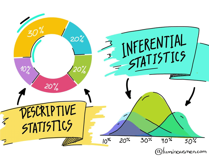
Descriptive statistics describes data (for example, a chart or graph) and inferential statistics allows you to make predictions (“inferences”) from that data. With inferential statistics, you take data from samples and make generalizations about a population
In this session we will explore inferential statistics.
2.0 Preparing Environment and Importing Data
2.0.1 Import Packages
# The modules we've seen before
import pandas as pd
import numpy as np
import matplotlib.pyplot as plt
import plotly.express as px
import seaborn as sns

# our stats modules
import random
import scipy.stats as stats
import statsmodels.api as sm
from statsmodels.formula.api import ols
import scipy
2.0.2 Load Dataset
For this session, we will use the truffletopia dataset
df = pd.read_csv('https://raw.githubusercontent.com/wesleybeckner/'\
                 'ds_for_engineers/main/data/truffle_margin/truffle_margin_customer.csv')
df
| Base Cake | Truffle Type | Primary Flavor | Secondary Flavor | Color Group | Customer | Date | KG | EBITDA/KG | |
|---|---|---|---|---|---|---|---|---|---|
| 0 | Butter | Candy Outer | Butter Pecan | Toffee | Taupe | Slugworth | 1/2020 | 53770.342593 | 0.500424 |
| 1 | Butter | Candy Outer | Ginger Lime | Banana | Amethyst | Slugworth | 1/2020 | 466477.578125 | 0.220395 |
| 2 | Butter | Candy Outer | Ginger Lime | Banana | Burgundy | Perk-a-Cola | 1/2020 | 80801.728070 | 0.171014 |
| 3 | Butter | Candy Outer | Ginger Lime | Banana | White | Fickelgruber | 1/2020 | 18046.111111 | 0.233025 |
| 4 | Butter | Candy Outer | Ginger Lime | Rum | Amethyst | Fickelgruber | 1/2020 | 19147.454268 | 0.480689 |
| ... | ... | ... | ... | ... | ... | ... | ... | ... | ... |
| 1663 | Tiramisu | Chocolate Outer | Doughnut | Pear | Amethyst | Fickelgruber | 12/2020 | 38128.802589 | 0.420111 |
| 1664 | Tiramisu | Chocolate Outer | Doughnut | Pear | Burgundy | Zebrabar | 12/2020 | 108.642857 | 0.248659 |
| 1665 | Tiramisu | Chocolate Outer | Doughnut | Pear | Teal | Zebrabar | 12/2020 | 3517.933333 | 0.378501 |
| 1666 | Tiramisu | Chocolate Outer | Doughnut | Rock and Rye | Amethyst | Slugworth | 12/2020 | 10146.898432 | 0.213149 |
| 1667 | Tiramisu | Chocolate Outer | Doughnut | Rock and Rye | Burgundy | Zebrabar | 12/2020 | 1271.904762 | 0.431813 |
1668 rows × 9 columns
descriptors = df.columns[:-2]
for col in df.columns[:-2]:
  print(col)
  print(df[col].unique())
  print()
Base Cake
['Butter' 'Cheese' 'Chiffon' 'Pound' 'Sponge' 'Tiramisu']

Truffle Type
['Candy Outer' 'Chocolate Outer' 'Jelly Filled']

Primary Flavor
['Butter Pecan' 'Ginger Lime' 'Margarita' 'Pear' 'Pink Lemonade'
 'Raspberry Ginger Ale' 'Sassafras' 'Spice' 'Wild Cherry Cream'
 'Cream Soda' 'Horchata' 'Kettle Corn' 'Lemon Bar' 'Orange Pineapple\tP'
 'Plum' 'Orange' 'Butter Toffee' 'Lemon' 'Acai Berry' 'Apricot'
 'Birch Beer' 'Cherry Cream Spice' 'Creme de Menthe' 'Fruit Punch'
 'Ginger Ale' 'Grand Mariner' 'Orange Brandy' 'Pecan' 'Toasted Coconut'
 'Watermelon' 'Wintergreen' 'Vanilla' 'Bavarian Cream' 'Black Licorice'
 'Caramel Cream' 'Cheesecake' 'Cherry Cola' 'Coffee' 'Irish Cream'
 'Lemon Custard' 'Mango' 'Sour' 'Amaretto' 'Blueberry' 'Butter Milk'
 'Chocolate Mint' 'Coconut' 'Dill Pickle' 'Gingersnap' 'Chocolate'
 'Doughnut']

Secondary Flavor
['Toffee' 'Banana' 'Rum' 'Tutti Frutti' 'Vanilla' 'Mixed Berry'
 'Whipped Cream' 'Apricot' 'Passion Fruit' 'Peppermint' 'Dill Pickle'
 'Black Cherry' 'Wild Cherry Cream' 'Papaya' 'Mango' 'Cucumber' 'Egg Nog'
 'Pear' 'Rock and Rye' 'Tangerine' 'Apple' 'Black Currant' 'Kiwi' 'Lemon'
 'Hazelnut' 'Butter Rum' 'Fuzzy Navel' 'Mojito' 'Ginger Beer']

Color Group
['Taupe' 'Amethyst' 'Burgundy' 'White' 'Black' 'Opal' 'Citrine' 'Rose'
 'Slate' 'Teal' 'Tiffany' 'Olive']

Customer
['Slugworth' 'Perk-a-Cola' 'Fickelgruber' 'Zebrabar' "Dandy's Candies"]

Date
['1/2020' '2/2020' '3/2020' '4/2020' '5/2020' '6/2020' '7/2020' '8/2020'
 '9/2020' '10/2020' '11/2020' '12/2020']
2.1 Navigating the Many Forms of Hypothesis Testing
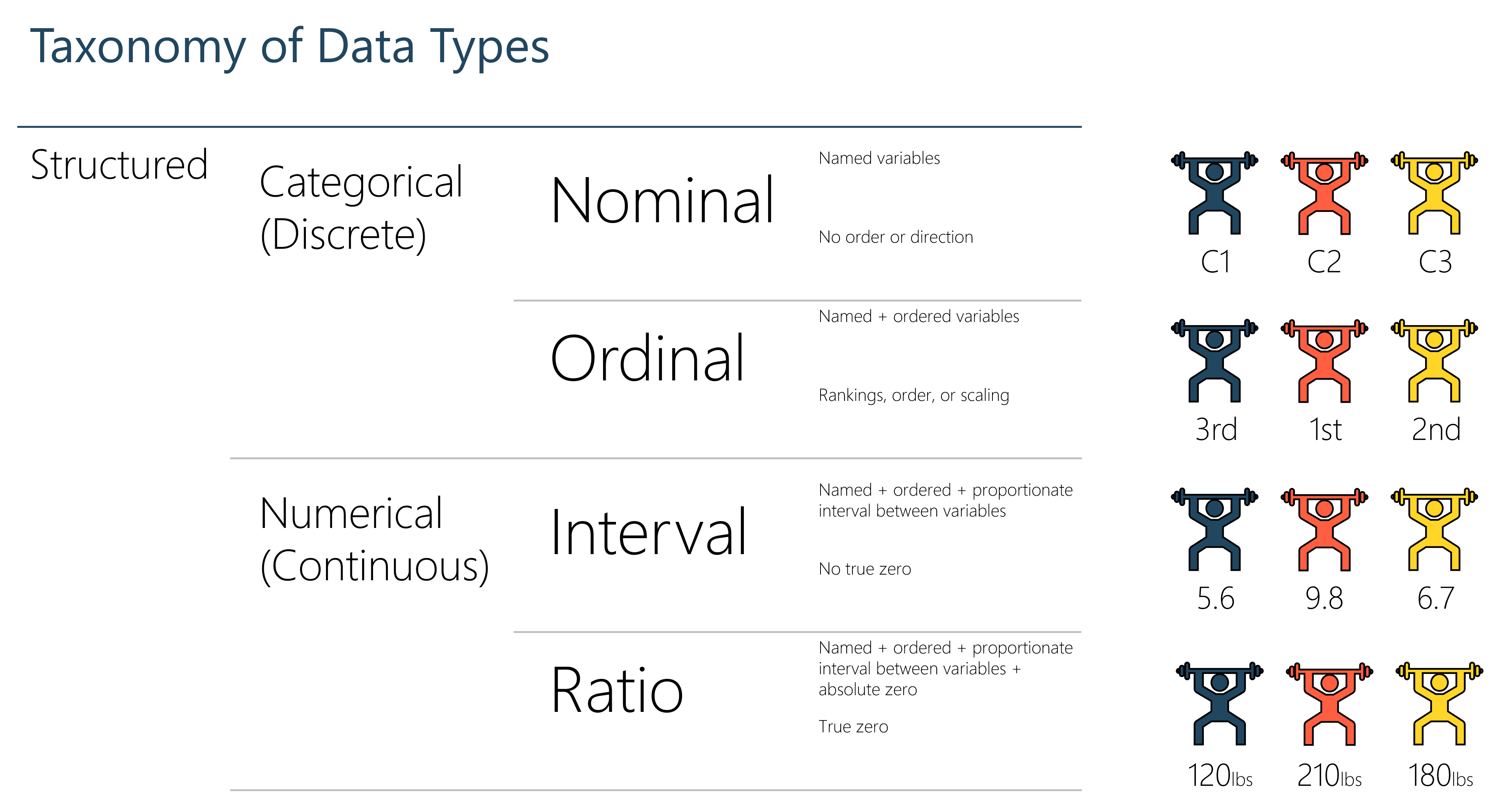
2.1.1 A Refresher on Data Types
Before we dive in, lets remind ourselves of the different data types. The acronym is NOIR: Nominal, Ordinal, Invterval, Ratio. And as we proceed along the acronym, more information is encapsulated in the data type. For this notebook the important distinction is between discrete (nominal/ordinal) and continuous (interval/ratio) data types. Depending on whether we are discrete or continuous, in either the target or predictor variable, we will proceed with a given set of hypothesis tests.
2.1.2 The Roadmap
Taking the taxonomy of datatypes and considering each of the predictor and outcome variables, we can concieve a roadmap
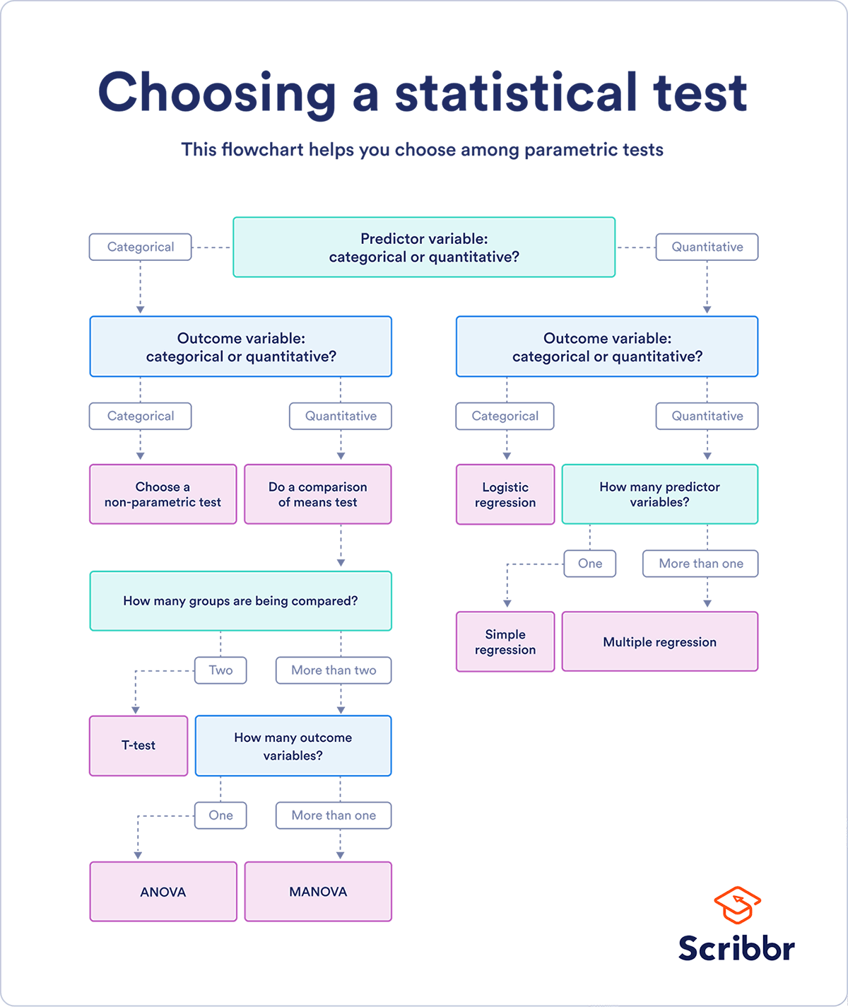
source: scribbr
The above diagram is imperfect (e.g. ANOVA is a comparison of variances, not of means) and non-comprehensive (e.g. where does moods median fit in this?). It will have to do until I make my own.
There are many modalities of hypothesis testing. We will not cover them all. The goal here, is to cover enough that you can leave this notebook with a basic idea of how the different tests relate to one another as well as their basic ingredients. What you will find is that among all these tests, a sample statistic is produced. The sample statistic itself is comprised typically of some expected value (for instance a mean) divided by a standard error of measure (for instance a standard deviation). In fact, we saw this in the previous notebook when discussing the confidence intervals around linear regression coefficients (and yes linear regression IS a form of hypothesis testing 😉)
In this notebook, we will touch on each of the following:
- Non-parametric tests
- Moods Median (Comparison of Medians)
- Kruskal-Wallis (Comparison of Medians, compare to ANOVA)
- Mann Whitney (Rank order test, compare to T-test)
- Comparison of means
- T-test
- Independent
- Equal Variances (students T-test)
- Unequal Variances (Welch's T-test)
- Dependent
- Independent
- T-test
- Comparison of variances
- Analysis of Variance (ANOVA)
- One Way ANOVA
- Two Way ANOVA
- MANOVA
- Factorial ANOVA
- Analysis of Variance (ANOVA)
When do I use each of these? We will talk about this as we proceed through the examples. Visit this Minitab Post for additional reading.
Finally, before we dive in and in the shadow of my making this hypothesis test decision tree a giant landmark on our journey, I invite you to read an excerpt from Chapter 1 of Statistical Rethinking (McElreath 2016). In this excerpt, McElreath tells a cautionary tale of using such roadmaps. Sorry McElreath. And if videos are more your bag, there you go.
For some, the toolbox of pre-manufactured golems is all they will ever need. Provided they stay within well-tested contexts, using only a few different procedures in appropriate tasks, a lot of good science can be completed. This is similar to how plumbers can do a lot of useful work without knowing much about fluid dynamics. Serious trouble begins when scholars move on to conducting innovative research, pushing the boundaries of their specialties. It's as if we got our hydraulic engineers by promoting plumbers.
Statistical Rethinking, McElreath 2016
2.2 What is Chi-Square?
You can use Chi-Square to test for a goodness of fit (whether a sample of data represents a distribution) or whether two variables are related (using a contingency table, which we will create below!)
Let's take an example. Imagine that you play Pokémon Go, in fact you love Pokémon Go. In your countless hours of study you've read that certain Pokémon will spawn under certain weather conditions. Rain, for instance, increases spawns of Water-, Electric, and Bug-type Pokémon. You decide to test this out. You record Pokémon sigtings in the same locations on days with and without rain and observe the following
random.seed(12)
types = ['electric', 'psychic', 'dark', 'bug', 'dragon', 'fire',
         'flying', 'ghost', 'grass', 'water']*1000
without_rain = random.sample(types, k=200)
types = ['electric', 'electric', 'electric', 'psychic', 'dark', 'bug', 'bug', 'bug', 'dragon', 'fire',
         'flying', 'ghost', 'grass', 'water', 'water', 'water']*1000
with_rain = random.sample(types, k=200)
given your observation of pokemon with rain (with_rain) and pokemon without rain (without_rain) how can you tell if these observations are statistically significant? i.e. that there actually is a difference in spawn rates for certain pokemon when it is and isn't raining? Enter the \(\chi^2\) test.
The chi-square test statistic:
Where \(O\) is the observed frequency and \(E\) is the expected frequency.
In our case, we are going to use the regular, sunny days as our expected values and the rainy days as our observed. See the data manipulation below:
rain = pd.DataFrame(np.unique(np.array(with_rain),
                       return_counts=True)).T
rain.columns=['type', 'O']
rain = rain.set_index('type')
sun = pd.DataFrame(np.unique(np.array(without_rain),
                       return_counts=True)).T
sun.columns=['type', 'E']
sun = sun.set_index('type')
table = rain.join(sun)
table
| O | E | |
|---|---|---|
| type | ||
| bug | 42 | 22 |
| dark | 13 | 22 |
| dragon | 15 | 19 |
| electric | 41 | 26 |
| fire | 10 | 26 |
| flying | 12 | 13 |
| ghost | 9 | 16 |
| grass | 12 | 12 |
| psychic | 11 | 21 |
| water | 35 | 23 |
Now that we have our observed and expected table we can compute the \(\chi^2\) test statistic
chi2 = ((table['O'] - table['E'])**2 / table['E']).sum()
print(f"the chi2 statistic: {chi2:.2f}")
the chi2 statistic: 55.37
Usually, a test statistic is not enough. We need to translate this into a probability; concretely, what is the probability of observing this test statistic under the null hypothesis? In order to answer this question we need to produce a distribution of test statistics. The steps are as follows:
- calculate the degrees of fredom (DoF)
- use the DoF to generate a probability distribution (PDF) for this particular test statistic (we will use scipy to do this)
- calculate (1 - the cumulative distribution (CDF) up to the test statistic)
- this value is the 1-sided probability of observing this test statistic or anything greater than it under the PDF
- multiply this value by 2 if we are interested in the 2-sided test (we usually are, unless we have a strong reason to believe the alternate hypothesis should appear on the right or left side of the null hypothesis)
- in our case, we believe that electric, bug, and water pokemon INCREASE with rain, so we will perform a 1-sided test
Our degrees of freedom can be calculated from the contingency table:
Which in our case DoF = 9
model = stats.chi2(df=9)
p = (1-model.cdf(chi2))
print(f"p value: {p:.2e}")
p value: 1.04e-08
We can verify our results with scipy's automagic:
stats.chisquare(f_obs = table['O'], f_exp = table['E'])
Power_divergenceResult(statistic=55.367939030839494, pvalue=1.0362934508722476e-08)
2.3 What is Mood's Median?
A special case of Pearon's Chi-Squared Test: We create a table that counts the observations above and below the global median for two or more groups. We then perform a chi-squared test of significance on this contingency table
Null hypothesis: the Medians are all equal
The chi-square test statistic:
Where \(O\) is the observed frequency and \(E\) is the expected frequency.
Let's take an example, say we have three shifts with the following production rates:
np.random.seed(7)
shift_one = [round(i) for i in np.random.normal(16, 3, 10)]
shift_two = [round(i) for i in np.random.normal(21, 3, 10)]
print(shift_one)
print(shift_two)
[21, 15, 16, 17, 14, 16, 16, 11, 19, 18]
[19, 20, 23, 20, 20, 17, 23, 21, 22, 16]
stat, p, m, table = scipy.stats.median_test(shift_one, shift_two, correction=False)
what is median_test returning?
print("The pearsons chi-square test statistic: {:.2f}".format(stat))
print("p-value of the test: {:.3f}".format(p))
print("the grand median: {}".format(m))
The pearsons chi-square test statistic: 7.20
p-value of the test: 0.007
the grand median: 18.5
Let's evaluate that test statistic ourselves by taking a look at the contingency table:
table
array([[2, 8],
       [8, 2]])
This is easier to make sense of if we order the shift times
shift_one.sort()
shift_one
[11, 14, 15, 16, 16, 16, 17, 18, 19, 21]
When we look at shift one, we see that 8 values are at or below the grand median.
shift_two.sort()
shift_two
[16, 17, 19, 20, 20, 20, 21, 22, 23, 23]
For shift two, only two are at or below the grand median.
Since the sample sizes are the same, the expected value for both groups is the same, 5 above and 5 below the grand median. The chi-square is then:
(2-5)**2/5 + (8-5)**2/5 + (8-5)**2/5 + (2-5)**2/5
7.2
Our p-value, or the probability of observing the null-hypothsis, is under 0.05 (at 0.007). We can conclude that these shift performances were drawn under seperate distributions.
For comparison, let's do this analysis again with shifts of equal performances
np.random.seed(3)
shift_three = [round(i) for i in np.random.normal(16, 3, 10)]
shift_four = [round(i) for i in np.random.normal(16, 3, 10)]
stat, p, m, table = scipy.stats.median_test(shift_three, shift_four,
                                            correction=False)
print("The pearsons chi-square test statistic: {:.2f}".format(stat))
print("p-value of the test: {:.3f}".format(p))
print("the grand median: {}".format(m))
The pearsons chi-square test statistic: 0.00
p-value of the test: 1.000
the grand median: 15.5
and the shift raw values:
shift_three.sort()
shift_four.sort()
print(shift_three)
print(shift_four)
[10, 14, 15, 15, 15, 16, 16, 16, 17, 21]
[11, 12, 13, 14, 15, 16, 19, 19, 19, 21]
table
array([[5, 5],
       [5, 5]])
2.3.1 When to Use Mood's?
Mood's Median Test is highly flexible but has the following assumptions:
- Considers only one categorical factor
- Response variable is continuous (our shift rates)
- Data does not need to be normally distributed
- But the distributions are similarly shaped
- Sample sizes can be unequal and small (less than 20 observations)
Other considerations:
- Not as powerful as Kruskal-Wallis Test but still useful for small sample sizes or when there are outliers
🏋️ Exercise 1: Use Mood's Median Test
Part A Perform moods median test on Base Cake (Categorical Variable) and EBITDA/KG (Continuous Variable) in Truffle data
We're also going to get some practice with pandas groupby.
# what is returned by this groupby?
gp = df.groupby('Base Cake')
How do we find out? We could iterate through it:
# seems to be a tuple of some sort
for i in gp:
  print(i)
  break
('Butter',      Base Cake     Truffle Type Primary Flavor Secondary Flavor Color Group  \
0       Butter      Candy Outer   Butter Pecan           Toffee       Taupe
1       Butter      Candy Outer    Ginger Lime           Banana    Amethyst
2       Butter      Candy Outer    Ginger Lime           Banana    Burgundy
3       Butter      Candy Outer    Ginger Lime           Banana       White
4       Butter      Candy Outer    Ginger Lime              Rum    Amethyst
...        ...              ...            ...              ...         ...
1562    Butter  Chocolate Outer           Plum     Black Cherry        Opal
1563    Butter  Chocolate Outer           Plum     Black Cherry       White
1564    Butter  Chocolate Outer           Plum            Mango       Black
1565    Butter     Jelly Filled         Orange         Cucumber    Amethyst
1566    Butter     Jelly Filled         Orange         Cucumber    Burgundy

             Customer     Date             KG  EBITDA/KG
0           Slugworth   1/2020   53770.342593   0.500424
1           Slugworth   1/2020  466477.578125   0.220395
2         Perk-a-Cola   1/2020   80801.728070   0.171014
3        Fickelgruber   1/2020   18046.111111   0.233025
4        Fickelgruber   1/2020   19147.454268   0.480689
...               ...      ...            ...        ...
1562     Fickelgruber  12/2020    9772.200521   0.158279
1563      Perk-a-Cola  12/2020   10861.245675  -0.159275
1564        Slugworth  12/2020    3578.592163   0.431328
1565        Slugworth  12/2020   21438.187500   0.105097
1566  Dandy's Candies  12/2020   15617.489115   0.185070

[456 rows x 9 columns])
# the first object appears to be the group
print(i[0])

# the second object appears to be the df belonging to that group
print(i[1])
Butter
     Base Cake     Truffle Type Primary Flavor Secondary Flavor Color Group  \
0       Butter      Candy Outer   Butter Pecan           Toffee       Taupe
1       Butter      Candy Outer    Ginger Lime           Banana    Amethyst
2       Butter      Candy Outer    Ginger Lime           Banana    Burgundy
3       Butter      Candy Outer    Ginger Lime           Banana       White
4       Butter      Candy Outer    Ginger Lime              Rum    Amethyst
...        ...              ...            ...              ...         ...
1562    Butter  Chocolate Outer           Plum     Black Cherry        Opal
1563    Butter  Chocolate Outer           Plum     Black Cherry       White
1564    Butter  Chocolate Outer           Plum            Mango       Black
1565    Butter     Jelly Filled         Orange         Cucumber    Amethyst
1566    Butter     Jelly Filled         Orange         Cucumber    Burgundy

             Customer     Date             KG  EBITDA/KG
0           Slugworth   1/2020   53770.342593   0.500424
1           Slugworth   1/2020  466477.578125   0.220395
2         Perk-a-Cola   1/2020   80801.728070   0.171014
3        Fickelgruber   1/2020   18046.111111   0.233025
4        Fickelgruber   1/2020   19147.454268   0.480689
...               ...      ...            ...        ...
1562     Fickelgruber  12/2020    9772.200521   0.158279
1563      Perk-a-Cola  12/2020   10861.245675  -0.159275
1564        Slugworth  12/2020    3578.592163   0.431328
1565        Slugworth  12/2020   21438.187500   0.105097
1566  Dandy's Candies  12/2020   15617.489115   0.185070

[456 rows x 9 columns]
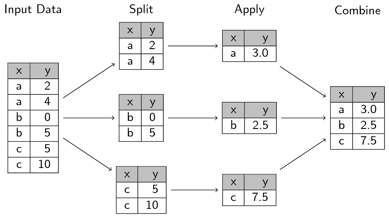
going back to our diagram from our earlier pandas session. It looks like whenever we split in the groupby method, we create separate dataframes as well as their group label:
Ok, so we know gp is separate dataframes. How do we turn them into arrays to then pass to median_test?
# complete this for loop
for i, j in gp:
  pass
  # turn 'EBITDA/KG' of j into an array using the .values attribute
  # print this to the screen
After you've completed the previous step, turn this into a list comprehension and pass the result to a variable called margins
# complete the code below
# margins = [# YOUR LIST COMPREHENSION HERE]
Remember the list unpacking we did for the tic tac toe project? We're going to do the same thing here. Unpack the margins list for median_test and run the cell below!
# complete the following line
# stat, p, m, table = scipy.stats.median_test(<UNPACK MARGINS HERE>, correction=False)

print("The pearsons chi-square test statistic: {:.2f}".format(stat))
print("p-value of the test: {:.2e}".format(p))
print("the grand median: {:.2e}".format(m))
The pearsons chi-square test statistic: 0.00
p-value of the test: 1.00e+00
the grand median: 1.55e+01
Part B View the distributions of the data using matplotlib and seaborn
What a fantastic statistical result we found! Can we affirm our result with some visualizations? I hope so! Create a boxplot below using pandas. In your call to df.boxplot() the by parameter should be set to Base Cake and the column parameter should be set to EBITDA/KG
# YOUR BOXPLOT HERE
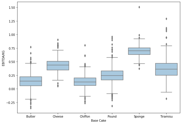
For comparison, I've shown the boxplot below using seaborn!
fig, ax = plt.subplots(figsize=(10,7))
ax = sns.boxplot(x='Base Cake', y='EBITDA/KG', data=df, color='#A0cbe8')
Part C Perform Moods Median on all the other groups
# Recall the other descriptors we have
descriptors
Index(['Base Cake', 'Truffle Type', 'Primary Flavor', 'Secondary Flavor',
       'Color Group', 'Customer', 'Date'],
      dtype='object')
for desc in descriptors:

  # YOUR CODE FORM MARGINS BELOW
  # margins = [<YOUR LIST COMPREHENSION>]

  # UNPACK MARGINS INTO MEDIAN_TEST
  # stat, p, m, table = scipy.stats.median_test(<YOUR UNPACKING METHOD>, correction=False)
  print(desc)
  print("The pearsons chi-square test statistic: {:.2f}".format(stat))
  print("p-value of the test: {:e}".format(p))
  print("the grand median: {}".format(m), end='\n\n')
Base Cake
The pearsons chi-square test statistic: 0.00
p-value of the test: 1.000000e+00
the grand median: 15.5

Truffle Type
The pearsons chi-square test statistic: 0.00
p-value of the test: 1.000000e+00
the grand median: 15.5

Primary Flavor
The pearsons chi-square test statistic: 0.00
p-value of the test: 1.000000e+00
the grand median: 15.5

Secondary Flavor
The pearsons chi-square test statistic: 0.00
p-value of the test: 1.000000e+00
the grand median: 15.5

Color Group
The pearsons chi-square test statistic: 0.00
p-value of the test: 1.000000e+00
the grand median: 15.5

Customer
The pearsons chi-square test statistic: 0.00
p-value of the test: 1.000000e+00
the grand median: 15.5

Date
The pearsons chi-square test statistic: 0.00
p-value of the test: 1.000000e+00
the grand median: 15.5
Part D Many boxplots
And finally, we will confirm these visually. Complete the Boxplot for each group:
for desc in descriptors:
  fig, ax = plt.subplots(figsize=(10,5))
  # sns.boxplot(x=<YOUR X VARIABLE HERE>, y='EBITDA/KG', data=df, color='#A0cbe8', ax=ax)


2.4 What is a T-test?
There are 1-sample and 2-sample T-tests
(note: we would use a 1-sample T-test just to determine if the sample mean is equal to a hypothesized population mean)
Within 2-sample T-tests we have independent and dependent T-tests (uncorrelated or correlated samples)
For independent, two-sample T-tests:
- Equal variance (or pooled) T-test
scipy.stats.ttest_ind(equal_var=True)- also called Student's T-test
- Unequal variance T-test
scipy.stats.ttest_ind(equal_var=False)- also called Welch's T-test
For dependent T-tests:
- Paired (or correlated) T-test
scipy.stats.ttest_rel- ex: patient symptoms before and after treatment
A full discussion on T-tests is outside the scope of this session, but we can refer to wikipedia for more information, including formulas on how each statistic is computed:
2.4.1 Demonstration of T-tests
We'll assume our shifts are of equal variance and proceed with the appropriate independent two-sample T-test...
print(shift_one)
print(shift_two)
[11, 14, 15, 16, 16, 16, 17, 18, 19, 21]
[16, 17, 19, 20, 20, 20, 21, 22, 23, 23]
To calculate the T-test, we follow a slightly different statistical formula:
where \(\mu\) are the means of the two groups, \(n\) are the sample sizes and \(s\) is the pooled standard deviation, also known as the cummulative variance (depending on if you square it or not):
where \(\sigma\) are the standard deviations. What you'll notice here is we are combining the two variances, we can only do this if we assume the variances are somewhat equal, this is known as the equal variances t-test.
mean_shift_one = np.mean(shift_one)
mean_shift_two = np.mean(shift_two)

print(mean_shift_one, mean_shift_two)
16.3 20.1
com_var = ((np.sum([(i - mean_shift_one)**2 for i in shift_one]) +
            np.sum([(i - mean_shift_two)**2 for i in shift_two])) /
            (len(shift_one) + len(shift_two)-2))
print(com_var)
6.5
T = (np.abs(mean_shift_one - mean_shift_two) / (
     np.sqrt(com_var/len(shift_one) +
     com_var/len(shift_two))))
T
3.3328204733667115
We see that this hand-computed result matches that of the scipy module:
scipy.stats.ttest_ind(shift_two, shift_one, equal_var=True)
Ttest_indResult(statistic=3.3328204733667115, pvalue=0.0037029158660758575)
2.5 What is ANOVA?
2.5.1 But First... What are F-statistics and the F-test?
The F-statistic is simply a ratio of two variances, or the ratio of mean squares
mean squares is the estimate of population variance that accounts for the degrees of freedom to compute that estimate.
We will explore this in the context of ANOVA
2.5.2 What is Analysis of Variance?
ANOVA uses the F-test to determine whether the variability between group means is larger than the variability within the groups. If that statistic is large enough, you can conclude that the means of the groups are not equal.
The caveat is that ANOVA tells us whether there is a difference in means but it does not tell us where the difference is. To find where the difference is between the groups, we have to conduct post-hoc tests.
There are two main types:
- One-way (one factor) and
- Two-way (two factor) where factor is an independent variable
| Ind A | Ind B | Dep |
|---|---|---|
| X | H | 10 |
| X | I | 12 |
| Y | I | 11 |
| Y | H | 20 |
ANOVA Hypotheses
- Null hypothesis: group means are equal
- Alternative hypothesis: at least one group mean is different from the other groups
ANOVA Assumptions
- Residuals (experimental error) are normally distributed (test with Shapiro-Wilk)
- Homogeneity of variances (variances are equal between groups) (test with Bartlett's)
- Observations are sampled independently from each other
- Note: ANOVA assumptions can be checked using test statistics (e.g. Shapiro-Wilk, Bartlett’s, Levene’s test) and the visual approaches such as residual plots (e.g. QQ-plots) and histograms.
Steps for ANOVA
- Check sample sizes: equal observations must be in each group
- Calculate Sum of Square between groups and within groups (\(SS_B, SS_E\))
- Calculate Mean Square between groups and within groups (\(MS_B, MS_E\))
- Calculate F value (\(MS_B/MS_E\))
This might be easier to see in a table:
| Source of Variation | degree of freedom (Df) | Sum of squares (SS) | Mean square (MS) | F value |
|---|---|---|---|---|
| Between Groups | Df_b = P-1 | SS_B | MS_B = SS_B / Df_B | MS_B / MS_E |
| Within Groups | Df_E = P(N-1) | SS_E | MS_E = SS_E / Df_E | |
| total | Df_T = PN-1 | SS_T |
Where:
Let's go back to our shift data to take an example:
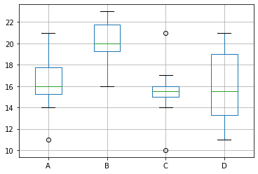
shifts = pd.DataFrame([shift_one, shift_two, shift_three, shift_four]).T
shifts.columns = ['A', 'B', 'C', 'D']
shifts.boxplot()
<AxesSubplot:>
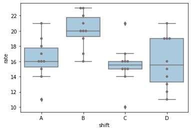
2.5.2.1 SNS Boxplot
this is another great way to view boxplot data. Notice how sns also shows us the raw data alongside the box and whiskers using a swarmplot.
shift_melt = pd.melt(shifts.reset_index(), id_vars=['index'],
                     value_vars=['A', 'B', 'C', 'D'])
shift_melt.columns = ['index', 'shift', 'rate']
ax = sns.boxplot(x='shift', y='rate', data=shift_melt, color='#A0cbe8')
ax = sns.swarmplot(x="shift", y="rate", data=shift_melt, color='#79706e')
Anyway back to ANOVA...
fvalue, pvalue = stats.f_oneway(shifts['A'],
                                shifts['B'],
                                shifts['C'],
                                shifts['D'])
print(fvalue, pvalue)
5.599173553719008 0.0029473487978665873
We can get this in the format of the table we saw above:
# get ANOVA table
import statsmodels.api as sm
from statsmodels.formula.api import ols

# Ordinary Least Squares (OLS) model
model = ols('rate ~ C(shift)', data=shift_melt).fit()
anova_table = sm.stats.anova_lm(model, typ=2)
anova_table
# output (ANOVA F and p value)
| sum_sq | df | F | PR(>F) | |
|---|---|---|---|---|
| C(shift) | 135.5 | 3.0 | 5.599174 | 0.002947 |
| Residual | 290.4 | 36.0 | NaN | NaN |
The Shapiro-Wilk test can be used to check the normal distribution of residuals. Null hypothesis: data is drawn from normal distribution.
w, pvalue = stats.shapiro(model.resid)
print(w, pvalue)
0.9750654697418213 0.5121709108352661
We can use Bartlett’s test to check the Homogeneity of variances. Null hypothesis: samples from populations have equal variances.
w, pvalue = stats.bartlett(shifts['A'],
                           shifts['B'],
                           shifts['C'],
                           shifts['D'])
print(w, pvalue)
1.3763632854696672 0.711084540821183
2.5.2.2 ANOVA Interpretation
The p value form ANOVA analysis is significant (p < 0.05) and we can conclude there are significant difference between the shifts. But we do not know which shift(s) are different. For this we need to perform a post hoc test. There are a multitude of these that are beyond the scope of this discussion (Tukey-kramer is one such test)

🍒 2.6 Enrichment: Evaluate statistical significance of product margin: a snake in the garden
2.6.1 Mood's Median on product descriptors
The first issue we run into with moods is... what?
Since Mood's is nonparametric, we can easily become overconfident in our results. Let's take an example, continuing with the Truffle Type column. Recall that there are 3 unique Truffle Types:
df['Truffle Type'].unique()
array(['Candy Outer', 'Chocolate Outer', 'Jelly Filled'], dtype=object)
We can loop through each group and compute the:
- Moods test (comparison of medians)
- Welch's T-test (unequal variances, comparison of means)
- Shapiro-Wilk test for normality
col = 'Truffle Type'
moodsdf = pd.DataFrame()
confidence_level = 0.01
welch_rej = mood_rej = shapiro_rej = False
for truff in df[col].unique():

  # for each
  group = df.loc[df[col] == truff]['EBITDA/KG']
  pop = df.loc[~(df[col] == truff)]['EBITDA/KG']
  stat, p, m, table = scipy.stats.median_test(group, pop)
  if p < confidence_level:
        mood_rej = True
  median = np.median(group)
  mean = np.mean(group)
  size = len(group)
  print("{}: N={}".format(truff, size))
  print("Moods Median Test")
  print("\tstatistic={:.2f}, pvalue={:.2e}".format(stat, p), end="\n")
  print(f"\treject: {mood_rej}")
  print("Welch's T-Test")
  print("\tstatistic={:.2f}, pvalue={:.2e}".format(*scipy.stats.ttest_ind(group, pop, equal_var=False)))
  welchp = scipy.stats.ttest_ind(group, pop, equal_var=False).pvalue
  if welchp < confidence_level:
        welch_rej = True
  print(f"\treject: {welch_rej}")
  print("Shapiro-Wilk")
  print("\tstatistic={:.2f}, pvalue={:.2e}".format(*stats.shapiro(group)))
  if stats.shapiro(group).pvalue < confidence_level:
    shapiro_rej = True
  print(f"\treject: {shapiro_rej}")
  print(end="\n\n")
  moodsdf = pd.concat([moodsdf,
                            pd.DataFrame([truff,
                                          stat, p, m, mean, median, size,
                                          welchp, table]).T])
moodsdf.columns = [col, 'pearsons_chi_square', 'p_value',
              'grand_median', 'group_mean', 'group_median', 'size', 'welch p',
              'table']
Candy Outer: N=288
Moods Median Test
    statistic=1.52, pvalue=2.18e-01
    reject: False
Welch's T-Test
    statistic=-2.76, pvalue=5.91e-03
    reject: True
Shapiro-Wilk
    statistic=0.96, pvalue=2.74e-07
    reject: True


Chocolate Outer: N=1356
Moods Median Test
    statistic=6.63, pvalue=1.00e-02
    reject: False
Welch's T-Test
    statistic=4.41, pvalue=1.19e-05
    reject: True
Shapiro-Wilk
    statistic=0.96, pvalue=6.30e-19
    reject: True


Jelly Filled: N=24
Moods Median Test
    statistic=18.64, pvalue=1.58e-05
    reject: True
Welch's T-Test
    statistic=-8.41, pvalue=7.93e-09
    reject: True
Shapiro-Wilk
    statistic=0.87, pvalue=6.56e-03
    reject: True
🙋♀️ Question 1: Moods Results on Truffle Type
What can we say about these results?
Recall that:
- Shapiro-Wilk Null Hypothesis: the distribution is normal
- Welch's T-test: requires that the distributions be normal
- Moods test: does not require normality in distributions
main conclusions: all the groups are non-normal and therefore welch's test is invalid. We saw that the Welch's test had much lower p-values than the Moods median test. This is good news! It means that our Moods test, while allowing for non-normality, is much more conservative in its test-statistic, and therefore was unable to reject the null hypothesis in the cases of the chocolate outer and candy outer groups
We can go ahead and repeat this analysis for all of our product categories:
df.columns[:5]
Index(['Base Cake', 'Truffle Type', 'Primary Flavor', 'Secondary Flavor',
       'Color Group'],
      dtype='object')
moodsdf = pd.DataFrame()
for col in df.columns[:5]:
  for truff in df[col].unique():
    group = df.loc[df[col] == truff]['EBITDA/KG']
    pop = df.loc[~(df[col] == truff)]['EBITDA/KG']
    stat, p, m, table = scipy.stats.median_test(group, pop)
    median = np.median(group)
    mean = np.mean(group)
    size = len(group)
    welchp = scipy.stats.ttest_ind(group, pop, equal_var=False).pvalue
    moodsdf = pd.concat([moodsdf,
                              pd.DataFrame([col, truff,
                                            stat, p, m, mean, median, size,
                                            welchp, table]).T])
moodsdf.columns = ['descriptor', 'group', 'pearsons_chi_square', 'p_value',
                'grand_median', 'group_mean', 'group_median', 'size', 'welch p',
                'table']
print(moodsdf.shape)
(101, 10)
moodsdf = moodsdf.loc[(moodsdf['p_value'] < confidence_level)].sort_values('group_median')

moodsdf = moodsdf.sort_values('group_median').reset_index(drop=True)
print(moodsdf.shape)
(57, 10)
moodsdf
| descriptor | group | pearsons_chi_square | p_value | grand_median | group_mean | group_median | size | welch p | table | |
|---|---|---|---|---|---|---|---|---|---|---|
| 0 | Secondary Flavor | Wild Cherry Cream | 6.798913 | 0.009121 | 0.216049 | -0.122491 | -0.15791 | 12 | 0.00001 | [[1, 833], [11, 823]] |
| 1 | Primary Flavor | Lemon Bar | 6.798913 | 0.009121 | 0.216049 | -0.122491 | -0.15791 | 12 | 0.00001 | [[1, 833], [11, 823]] |
| 2 | Primary Flavor | Orange Pineapple\tP | 18.643248 | 0.000016 | 0.216049 | 0.016747 | 0.002458 | 24 | 0.0 | [[1, 833], [23, 811]] |
| 3 | Secondary Flavor | Papaya | 18.643248 | 0.000016 | 0.216049 | 0.016747 | 0.002458 | 24 | 0.0 | [[1, 833], [23, 811]] |
| 4 | Primary Flavor | Cherry Cream Spice | 10.156401 | 0.001438 | 0.216049 | 0.018702 | 0.009701 | 12 | 0.000001 | [[0, 834], [12, 822]] |
| 5 | Secondary Flavor | Cucumber | 18.643248 | 0.000016 | 0.216049 | 0.051382 | 0.017933 | 24 | 0.0 | [[1, 833], [23, 811]] |
| 6 | Truffle Type | Jelly Filled | 18.643248 | 0.000016 | 0.216049 | 0.051382 | 0.017933 | 24 | 0.0 | [[1, 833], [23, 811]] |
| 7 | Primary Flavor | Orange | 18.643248 | 0.000016 | 0.216049 | 0.051382 | 0.017933 | 24 | 0.0 | [[1, 833], [23, 811]] |
| 8 | Primary Flavor | Toasted Coconut | 15.261253 | 0.000094 | 0.216049 | 0.037002 | 0.028392 | 24 | 0.0 | [[2, 832], [22, 812]] |
| 9 | Primary Flavor | Wild Cherry Cream | 6.798913 | 0.009121 | 0.216049 | 0.047647 | 0.028695 | 12 | 0.00038 | [[1, 833], [11, 823]] |
| 10 | Secondary Flavor | Apricot | 15.261253 | 0.000094 | 0.216049 | 0.060312 | 0.037422 | 24 | 0.0 | [[2, 832], [22, 812]] |
| 11 | Primary Flavor | Kettle Corn | 29.062065 | 0.0 | 0.216049 | 0.055452 | 0.045891 | 60 | 0.0 | [[9, 825], [51, 783]] |
| 12 | Primary Flavor | Acai Berry | 18.643248 | 0.000016 | 0.216049 | 0.036505 | 0.049466 | 24 | 0.0 | [[1, 833], [23, 811]] |
| 13 | Primary Flavor | Pink Lemonade | 10.156401 | 0.001438 | 0.216049 | 0.039862 | 0.056349 | 12 | 0.000011 | [[0, 834], [12, 822]] |
| 14 | Secondary Flavor | Black Cherry | 58.900366 | 0.0 | 0.216049 | 0.055975 | 0.062898 | 96 | 0.0 | [[11, 823], [85, 749]] |
| 15 | Primary Flavor | Watermelon | 15.261253 | 0.000094 | 0.216049 | 0.04405 | 0.067896 | 24 | 0.0 | [[2, 832], [22, 812]] |
| 16 | Primary Flavor | Sassafras | 6.798913 | 0.009121 | 0.216049 | 0.072978 | 0.074112 | 12 | 0.000059 | [[1, 833], [11, 823]] |
| 17 | Primary Flavor | Plum | 34.851608 | 0.0 | 0.216049 | 0.084963 | 0.079993 | 72 | 0.0 | [[11, 823], [61, 773]] |
| 18 | Secondary Flavor | Dill Pickle | 10.156401 | 0.001438 | 0.216049 | 0.037042 | 0.082494 | 12 | 0.000007 | [[0, 834], [12, 822]] |
| 19 | Primary Flavor | Horchata | 10.156401 | 0.001438 | 0.216049 | 0.037042 | 0.082494 | 12 | 0.000007 | [[0, 834], [12, 822]] |
| 20 | Primary Flavor | Lemon Custard | 12.217457 | 0.000473 | 0.216049 | 0.079389 | 0.087969 | 24 | 0.000006 | [[3, 831], [21, 813]] |
| 21 | Primary Flavor | Fruit Punch | 10.156401 | 0.001438 | 0.216049 | 0.078935 | 0.090326 | 12 | 0.000076 | [[0, 834], [12, 822]] |
| 22 | Base Cake | Chiffon | 117.046226 | 0.0 | 0.216049 | 0.127851 | 0.125775 | 288 | 0.0 | [[60, 774], [228, 606]] |
| 23 | Base Cake | Butter | 134.36727 | 0.0 | 0.216049 | 0.142082 | 0.139756 | 456 | 0.0 | [[122, 712], [334, 500]] |
| 24 | Secondary Flavor | Banana | 10.805348 | 0.001012 | 0.216049 | 0.163442 | 0.15537 | 60 | 0.0 | [[17, 817], [43, 791]] |
| 25 | Primary Flavor | Cream Soda | 9.511861 | 0.002041 | 0.216049 | 0.150265 | 0.163455 | 24 | 0.000002 | [[4, 830], [20, 814]] |
| 26 | Secondary Flavor | Peppermint | 9.511861 | 0.002041 | 0.216049 | 0.150265 | 0.163455 | 24 | 0.000002 | [[4, 830], [20, 814]] |
| 27 | Primary Flavor | Grand Mariner | 10.581767 | 0.001142 | 0.216049 | 0.197463 | 0.165529 | 72 | 0.000829 | [[22, 812], [50, 784]] |
| 28 | Color Group | Amethyst | 20.488275 | 0.000006 | 0.216049 | 0.195681 | 0.167321 | 300 | 0.0 | [[114, 720], [186, 648]] |
| 29 | Color Group | Burgundy | 10.999677 | 0.000911 | 0.216049 | 0.193048 | 0.171465 | 120 | 0.000406 | [[42, 792], [78, 756]] |
| 30 | Color Group | White | 35.76526 | 0.0 | 0.216049 | 0.19 | 0.177264 | 432 | 0.0 | [[162, 672], [270, 564]] |
| 31 | Primary Flavor | Ginger Lime | 7.835047 | 0.005124 | 0.216049 | 0.21435 | 0.183543 | 84 | 0.001323 | [[29, 805], [55, 779]] |
| 32 | Primary Flavor | Mango | 11.262488 | 0.000791 | 0.216049 | 0.28803 | 0.245049 | 132 | 0.009688 | [[85, 749], [47, 787]] |
| 33 | Color Group | Opal | 11.587164 | 0.000664 | 0.216049 | 0.317878 | 0.259304 | 324 | 0.0 | [[190, 644], [134, 700]] |
| 34 | Secondary Flavor | Apple | 27.283292 | 0.0 | 0.216049 | 0.326167 | 0.293876 | 36 | 0.001176 | [[34, 800], [2, 832]] |
| 35 | Secondary Flavor | Tangerine | 32.626389 | 0.0 | 0.216049 | 0.342314 | 0.319273 | 48 | 0.000113 | [[44, 790], [4, 830]] |
| 36 | Secondary Flavor | Black Currant | 34.778391 | 0.0 | 0.216049 | 0.357916 | 0.332449 | 36 | 0.0 | [[36, 798], [0, 834]] |
| 37 | Secondary Flavor | Pear | 16.614303 | 0.000046 | 0.216049 | 0.373034 | 0.33831 | 60 | 0.000031 | [[46, 788], [14, 820]] |
| 38 | Primary Flavor | Vanilla | 34.778391 | 0.0 | 0.216049 | 0.378053 | 0.341626 | 36 | 0.000001 | [[36, 798], [0, 834]] |
| 39 | Color Group | Citrine | 10.156401 | 0.001438 | 0.216049 | 0.390728 | 0.342512 | 12 | 0.001925 | [[12, 822], [0, 834]] |
| 40 | Color Group | Teal | 13.539679 | 0.000234 | 0.216049 | 0.323955 | 0.3446 | 96 | 0.00121 | [[66, 768], [30, 804]] |
| 41 | Base Cake | Tiramisu | 52.360619 | 0.0 | 0.216049 | 0.388267 | 0.362102 | 144 | 0.0 | [[114, 720], [30, 804]] |
| 42 | Primary Flavor | Doughnut | 74.935256 | 0.0 | 0.216049 | 0.439721 | 0.379361 | 108 | 0.0 | [[98, 736], [10, 824]] |
| 43 | Secondary Flavor | Ginger Beer | 22.363443 | 0.000002 | 0.216049 | 0.444895 | 0.382283 | 24 | 0.000481 | [[24, 810], [0, 834]] |
| 44 | Color Group | Rose | 18.643248 | 0.000016 | 0.216049 | 0.42301 | 0.407061 | 24 | 0.000062 | [[23, 811], [1, 833]] |
| 45 | Base Cake | Cheese | 66.804744 | 0.0 | 0.216049 | 0.450934 | 0.435638 | 84 | 0.0 | [[79, 755], [5, 829]] |
| 46 | Primary Flavor | Butter Toffee | 60.181468 | 0.0 | 0.216049 | 0.50366 | 0.456343 | 60 | 0.0 | [[60, 774], [0, 834]] |
| 47 | Color Group | Slate | 10.156401 | 0.001438 | 0.216049 | 0.540214 | 0.483138 | 12 | 0.000017 | [[12, 822], [0, 834]] |
| 48 | Primary Flavor | Gingersnap | 22.363443 | 0.000002 | 0.216049 | 0.643218 | 0.623627 | 24 | 0.0 | [[24, 810], [0, 834]] |
| 49 | Primary Flavor | Dill Pickle | 22.363443 | 0.000002 | 0.216049 | 0.642239 | 0.655779 | 24 | 0.0 | [[24, 810], [0, 834]] |
| 50 | Color Group | Olive | 44.967537 | 0.0 | 0.216049 | 0.637627 | 0.670186 | 60 | 0.0 | [[56, 778], [4, 830]] |
| 51 | Primary Flavor | Butter Milk | 10.156401 | 0.001438 | 0.216049 | 0.699284 | 0.688601 | 12 | 0.0 | [[12, 822], [0, 834]] |
| 52 | Base Cake | Sponge | 127.156266 | 0.0 | 0.216049 | 0.698996 | 0.699355 | 120 | 0.0 | [[120, 714], [0, 834]] |
| 53 | Primary Flavor | Chocolate Mint | 10.156401 | 0.001438 | 0.216049 | 0.685546 | 0.699666 | 12 | 0.0 | [[12, 822], [0, 834]] |
| 54 | Primary Flavor | Coconut | 10.156401 | 0.001438 | 0.216049 | 0.732777 | 0.717641 | 12 | 0.0 | [[12, 822], [0, 834]] |
| 55 | Primary Flavor | Blueberry | 22.363443 | 0.000002 | 0.216049 | 0.759643 | 0.72536 | 24 | 0.0 | [[24, 810], [0, 834]] |
| 56 | Primary Flavor | Amaretto | 10.156401 | 0.001438 | 0.216049 | 0.782156 | 0.764845 | 12 | 0.0 | [[12, 822], [0, 834]] |
2.6.2 Broad Analysis of Categories: ANOVA
Recall our "melted" shift data. It will be useful to think of getting our Truffle data in this format:
shift_melt.head()
| index | shift | rate | |
|---|---|---|---|
| 0 | 0 | A | 15 |
| 1 | 1 | A | 15 |
| 2 | 2 | A | 15 |
| 3 | 3 | A | 16 |
| 4 | 4 | A | 17 |
df.columns = df.columns.str.replace(' ', '_')
df.columns = df.columns.str.replace('/', '_')
# get ANOVA table
# Ordinary Least Squares (OLS) model
model = ols('EBITDA_KG ~ C(Truffle_Type)', data=df).fit()
anova_table = sm.stats.anova_lm(model, typ=2)
anova_table
# output (ANOVA F and p value)
| sum_sq | df | F | PR(>F) | |
|---|---|---|---|---|
| C(Truffle_Type) | 1.250464 | 2.0 | 12.882509 | 0.000003 |
| Residual | 80.808138 | 1665.0 | NaN | NaN |
Recall the Shapiro-Wilk test can be used to check the normal distribution of residuals. Null hypothesis: data is drawn from normal distribution.
w, pvalue = stats.shapiro(model.resid)
print(w, pvalue)
0.9576056599617004 1.2598073820281984e-21
And the Bartlett’s test to check the Homogeneity of variances. Null hypothesis: samples from populations have equal variances.
gb = df.groupby('Truffle_Type')['EBITDA_KG']
gb
<pandas.core.groupby.generic.SeriesGroupBy object at 0x7fafac7cfd10>
w, pvalue = stats.bartlett(*[gb.get_group(x) for x in gb.groups])
print(w, pvalue)
109.93252546442552 1.344173733366234e-24
Wow it looks like our data is not drawn from a normal distribution! Let's check this for other categories...
We can wrap these in a for loop:
for col in df.columns[:5]:
  print(col)
  model = ols('EBITDA_KG ~ C({})'.format(col), data=df).fit()
  anova_table = sm.stats.anova_lm(model, typ=2)
  display(anova_table)
  w, pvalue = stats.shapiro(model.resid)
  print("Shapiro: ", w, pvalue)
  gb = df.groupby(col)['EBITDA_KG']
  w, pvalue = stats.bartlett(*[gb.get_group(x) for x in gb.groups])
  print("Bartlett: ", w, pvalue)
  print()
Base_Cake
| sum_sq | df | F | PR(>F) | |
|---|---|---|---|---|
| C(Base_Cake) | 39.918103 | 5.0 | 314.869955 | 1.889884e-237 |
| Residual | 42.140500 | 1662.0 | NaN | NaN |
Shapiro:  0.9634131193161011 4.1681337029688696e-20
Bartlett:  69.83288886114195 1.1102218566053728e-13

Truffle_Type
| sum_sq | df | F | PR(>F) | |
|---|---|---|---|---|
| C(Truffle_Type) | 1.250464 | 2.0 | 12.882509 | 0.000003 |
| Residual | 80.808138 | 1665.0 | NaN | NaN |
Shapiro:  0.9576056599617004 1.2598073820281984e-21
Bartlett:  109.93252546442552 1.344173733366234e-24

Primary_Flavor
| sum_sq | df | F | PR(>F) | |
|---|---|---|---|---|
| C(Primary_Flavor) | 50.270639 | 50.0 | 51.143649 | 1.153434e-292 |
| Residual | 31.787964 | 1617.0 | NaN | NaN |
Shapiro:  0.948470413684845 9.90281706784179e-24
Bartlett:  210.15130419114894 1.5872504991231547e-21

Secondary_Flavor
| sum_sq | df | F | PR(>F) | |
|---|---|---|---|---|
| C(Secondary_Flavor) | 15.088382 | 28.0 | 13.188089 | 1.929302e-54 |
| Residual | 66.970220 | 1639.0 | NaN | NaN |
Shapiro:  0.9548103213310242 2.649492974953278e-22
Bartlett:  420.6274502894803 1.23730070350945e-71

Color_Group
| sum_sq | df | F | PR(>F) | |
|---|---|---|---|---|
| C(Color_Group) | 16.079685 | 11.0 | 36.689347 | 6.544980e-71 |
| Residual | 65.978918 | 1656.0 | NaN | NaN |
Shapiro:  0.969061017036438 1.8926407335144587e-18
Bartlett:  136.55525281340468 8.164787784033709e-24
2.6.3 Visual Analysis of Residuals: QQ-Plots
This can be distressing and is often why we want visual methods to see what is going on with our data!
model = ols('EBITDA_KG ~ C(Truffle_Type)', data=df).fit()

#create instance of influence
influence = model.get_influence()

#obtain standardized residuals
standardized_residuals = influence.resid_studentized_internal

# res.anova_std_residuals are standardized residuals obtained from ANOVA (check above)
sm.qqplot(standardized_residuals, line='45')
plt.xlabel("Theoretical Quantiles")
plt.ylabel("Standardized Residuals")
plt.show()

# histogram
plt.hist(model.resid, bins='auto', histtype='bar', ec='k')
plt.xlabel("Residuals")
plt.ylabel('Frequency')
plt.show()
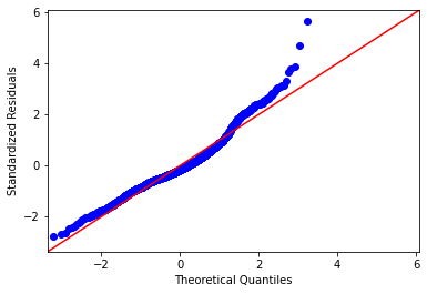
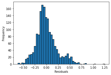
We see that a lot of our data is swayed by extremely high and low values, so what can we conclude?
You need the right test statistic for the right job, in this case, we are littered with unequal variance in our groupings so we use the moods median and welch (unequal variance t-test) to make conclusions about our data